Reorientation and fragmentation#

One coherent story: under load, grains reorient; that reorientation fragments them into orientation sub-grains; and the grains that fragment the most are the rare events. The same two classes drive all of it – OrientationTracker builds the IPF trajectories and FragmentationAnalyzer does the segmentation, split detection, and per-grain fragment counts.

Needs: NEML2 v3 (orientation math) and networkit (segmentation); no external binaries. The simulation parts run on the shipped real CPFE run mwe_data/cpfe_ff_fragmentation; the experiment parts on the synthetic split series mwe_data/synthetic_split_{ff,nf,ebsd}.

1. Simulation: grains reorient under load#

OrientationTracker().simulation_grain_tracks reads each grain’s ori_rodrigues (neml2 MRP) block time series; plot_ipf_orientation_tracking draws one IPF triangle with a start dot and a reorientation arrow per grain.

[1]:

import numpy as np
from graintrace.simulation_postprocessing import SimulationResults, FieldFileNaming
from graintrace.ipf_orientation_tracking import OrientationTracker
from graintrace.fragmentation import FragmentationAnalyzer
from graintrace import plot_postprocessing as pp

naming = FieldFileNaming(prefix="out_element_centroid", index_width=4, sep="_", suffix=".csv")
res = SimulationResults(
    "../../mwe_data/cpfe_ff_fragmentation/out.csv",
    "../../mwe_data/cpfe_ff_fragmentation/mesh_out", field_naming=naming)
tracker, analyzer = OrientationTracker(), FragmentationAnalyzer()
steps = sorted(res.field_files.keys())
tracks = tracker.simulation_grain_tracks(res, grain_ids=list(range(1, 11)), steps=steps)
pp.plot_ipf_orientation_tracking(tracks, angle_convention="mrp", output_folder="out")

/workspace/personal/repos/graintrace/.venv/lib/python3.12/site-packages/tqdm/auto.py:21: TqdmWarning: IProgress not found. Please update jupyter and ipywidgets. See https://ipywidgets.readthedocs.io/en/stable/user_install.html
  from .autonotebook import tqdm as notebook_tqdm

[1]:

PosixPath('out/ipf_orientation_tracking.png')

[2]:

from IPython.display import Image

# plot_ipf_orientation_tracking writes to output_folder and does not call plt.show(),
# so load the PNG it just wrote.
Image("out/ipf_orientation_tracking.png")

[2]:

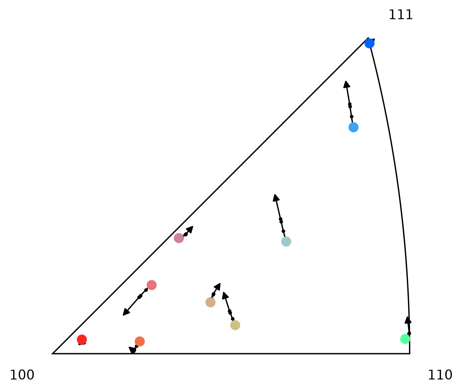
../_images/tutorials_reorientation-fragmentation_3_0.png

Each dot is a grain’s starting orientation, coloured by the standard IPF key; the black line is its path through the load steps and the arrowhead is where it ended. Short arrows are grains rotating barely at all, long ones are grains whose lattice is being dragged around by slip. This is the per-grain average — section 2 opens each grain up to see whether its elements moved together.

2. Simulation: reorientation to fragmentation (the 1x2 figure)#

FragmentationAnalyzer().grain_fragments re-segments each grain’s elements by orientation into sub-grains. For intragranular data pass a fixed low Leiden gamma (here gamma=0.25; the gamma-by-percolation sweep is only for large many-grain NF/EBSD, and gamma=0.1 under-splits – it leaves most grains whole). Leiden alone will still chop a smooth intragranular gradient into several near-identical communities, so min_subgrain_miso_deg (here 1°) imposes a minimum sub-grain misorientation: after Leiden, fragments whose (symmetry-aware) mean orientations are closer than that are merged, so only genuine sub-grains – separated by a real low-angle sub-boundary – survive as distinct fragments. The signature figure puts the two views side by side on the real CPFE data and links them by two channels:

LEFT – every element of each grain (OrientationTracker().simulation_element_tracks), so the width of each fan is that grain’s intragranular reorientation spread. Lines are thin and headless (line_width=0.8, show_arrow=False) because the panel is crowded.
RIGHT – the resulting sub-grain forks (plot_ipf_fragmentation_tracking): the parent trajectory (neutral gray) forks at its split point into one child per fragment, small arrowhead.

The linking channels are color and line style, both keyed to a per-grain fragment index. Color comes from a dark, high-contrast qualitative palette (ColorBrewer Dark2) so a grain’s sub-grains contrast sharply – pass a per-element arrow_color list on the left and the per-child child_colors (with parent_color for the gray parent) on the right. The palette is reused across grains (grains are told apart by their IPF position, sub-grains by color), and the start dots are drawn neutral black (start_color="black"). Line style (-, --, -., :) reinforces the same fragment index in the crowded left panel. So a fork on the right and the element cloud that formed it on the left share both color and style. Both plotters take a shared ax (returning it instead of saving) plus line_width, arrow_scale, show_arrow, and label_fontsize. (arrow_color="ipf_final" is also available, tinting each track by the IPF color of its endpoint, when you prefer color to encode the final orientation.)

[3]:

import matplotlib.pyplot as plt

last = steps[-1]
ori_cols = ["ori_rodrigues_x", "ori_rodrigues_y", "ori_rodrigues_z"]
grains = list(range(1, 11))
STYLES = ["-", "--", "-.", ":"]
# dark, high-contrast qualitative palette (ColorBrewer Dark2) keyed by fragment
COLORS = ["#1b9e77", "#d95f02", "#7570b3", "#e7298a", "#66a61e", "#a6761d"]

# min_subgrain_miso_deg=1.0: only keep a split if the sub-grains differ by >1 deg, so a
# smooth intragranular gradient is not chopped into near-identical fragments (the mean used
# for the merge and the fork endpoints is a symmetry-aware quaternion mean).
frags_df, per_elem = analyzer.grain_fragments(
    res, last, tol_deg=5.0, min_subgrain_miso_deg=1.0, seg_kwargs={"gamma": 0.25})

# per-grain fragment-label -> (style, color): sub-grains of one grain contrast sharply
frag_style, frag_color = {}, {}
for g in grains:
    labs = sorted(l for l in per_elem.values() if l.startswith(f"{g}."))
    frag_style[g] = {lab: STYLES[i % len(STYLES)] for i, lab in enumerate(labs)}
    frag_color[g] = {lab: COLORS[i % len(COLORS)] for i, lab in enumerate(labs)}

# LEFT: every element of each grain, colored + styled by the fragment it belongs to
df0 = res.load_field_data(steps[0])
blk0 = np.rint(df0["block_id"].to_numpy()).astype(int)
left_tracks, left_styles, left_colors = [], [], []
for g in grains:
    eids = df0.loc[blk0 == g, "id"].astype(int).tolist()
    for eid, tr in zip(eids, tracker.simulation_element_tracks(res, element_ids=eids, steps=steps)):
        lab = per_elem.get(eid)
        left_tracks.append(tr)
        left_styles.append(frag_style[g].get(lab, "-"))
        left_colors.append(frag_color[g].get(lab, "0.35"))

# RIGHT: parent (pre-last) forks into per-fragment children at the last step
# (mean_orientation_mrp is symmetry-aware -- pass the analyzer's symmetry)
last_df = res.load_field_data(last).set_index("id")
branches, child_styles, child_colors = [], [], []
for g in grains:
    parent = np.asarray([
        analyzer.mean_orientation_mrp(
            df[np.rint(df["block_id"].to_numpy()).astype(int) == g][ori_cols].to_numpy(),
            analyzer.symmetry)
        for df in (res.load_field_data(int(s)) for s in steps[:-1])])
    labs = sorted(frag_style[g])
    children = [analyzer.mean_orientation_mrp(
        last_df.loc[[e for e, l in per_elem.items() if l == lab], ori_cols].to_numpy(),
        analyzer.symmetry)[None, :] for lab in labs]
    branches.append((parent, children))
    child_styles.append([frag_style[g][lab] for lab in labs])
    child_colors.append([frag_color[g][lab] for lab in labs])

# color = dark categorical fragment color (a grain's sub-grains contrast), black start
# dots, gray parent, no legend; line style reinforces the fragment.
fig, (axL, axR) = plt.subplots(1, 2, figsize=(14, 7))
pp.plot_ipf_orientation_tracking(left_tracks, angle_convention="mrp", arrow_color=left_colors,
    start_color="black", line_style=left_styles, line_width=0.8, show_arrow=False,
    label_fontsize=18, ax=axL)
pp.plot_ipf_fragmentation_tracking(branches, angle_convention="mrp", child_colors=child_colors,
    parent_color="0.35", start_color="black", child_line_styles=child_styles, line_width=2.0,
    arrow_scale=12, show_arrow=True, label_fontsize=18, ax=axR)
fig.tight_layout()
fig.savefig("out/reorientation_vs_fragmentation.png")


=== Running GraphSpatialCluster ===

Data loaded.

Building graph with mode: knn

Building edges from nodes: 100%|██████████| 161/161 [00:00<00:00, 94155.46it/s]

Graph is built. Number of edges: 1089, Number of nodes: 161, Number of features: 3

Computing edge distances with metric: misorientation

Edge distances: 100%|██████████| 1089/1089 [00:00<00:00, 4081.71edge/s]


Keeping edges with distance <= 0.08726646259971647
Updated number of edges: 1064

Converting edge distances to weights

Removing edges to keep only top 12 weights per node
Updated number of edges: 1021

Saving checkpoint: /tmp/segori_k0y1akkj/seg_ckpt (edges/weights/meta)

Segmenting graph with method: leiden
Segmenter parameters: {'gamma': 0.25}

  NetworKit Leiden threads set to 1 (machine max 1)

=== Running GraphSpatialCluster ===

Data loaded.

Building graph with mode: knn

Building edges from nodes: 100%|██████████| 61/61 [00:00<00:00, 57702.42it/s]

Graph is built. Number of edges: 395, Number of nodes: 61, Number of features: 3

Computing edge distances with metric: misorientation

Edge distances: 100%|██████████| 395/395 [00:00<00:00, 7598.90edge/s]


Keeping edges with distance <= 0.08726646259971647
Updated number of edges: 395

Converting edge distances to weights

Removing edges to keep only top 12 weights per node
Updated number of edges: 379

Saving checkpoint: /tmp/segori_to8jrdva/seg_ckpt (edges/weights/meta)

Segmenting graph with method: leiden
Segmenter parameters: {'gamma': 0.25}
  NetworKit Leiden threads set to 1 (machine max 1)

=== Running GraphSpatialCluster ===

Data loaded.

Building graph with mode: knn

Building edges from nodes: 100%|██████████| 96/96 [00:00<00:00, 72380.58it/s]

Graph is built. Number of edges: 638, Number of nodes: 96, Number of features: 3

Computing edge distances with metric: misorientation

Edge distances: 100%|██████████| 638/638 [00:00<00:00, 7992.73edge/s]


Keeping edges with distance <= 0.08726646259971647
Updated number of edges: 527

Converting edge distances to weights

Removing edges to keep only top 12 weights per node
Updated number of edges: 524

Saving checkpoint: /tmp/segori_i4oa8e7q/seg_ckpt (edges/weights/meta)

Segmenting graph with method: leiden
Segmenter parameters: {'gamma': 0.25}
  NetworKit Leiden threads set to 1 (machine max 1)

=== Running GraphSpatialCluster ===

Data loaded.

Building graph with mode: knn

Building edges from nodes: 100%|██████████| 98/98 [00:00<00:00, 74626.32it/s]

Graph is built. Number of edges: 659, Number of nodes: 98, Number of features: 3

Computing edge distances with metric: misorientation

Edge distances: 100%|██████████| 659/659 [00:00<00:00, 8019.47edge/s]


Keeping edges with distance <= 0.08726646259971647
Updated number of edges: 615

Converting edge distances to weights

Removing edges to keep only top 12 weights per node
Updated number of edges: 590

Saving checkpoint: /tmp/segori_ly_x7587/seg_ckpt (edges/weights/meta)

Segmenting graph with method: leiden
Segmenter parameters: {'gamma': 0.25}
  NetworKit Leiden threads set to 1 (machine max 1)

=== Running GraphSpatialCluster ===

Data loaded.

Building graph with mode: knn

Building edges from nodes: 100%|██████████| 119/119 [00:00<00:00, 92004.09it/s]

Graph is built. Number of edges: 803, Number of nodes: 119, Number of features: 3

Computing edge distances with metric: misorientation

Edge distances: 100%|██████████| 803/803 [00:00<00:00, 7890.57edge/s]


Keeping edges with distance <= 0.08726646259971647
Updated number of edges: 765

Converting edge distances to weights

Removing edges to keep only top 12 weights per node
Updated number of edges: 735

Saving checkpoint: /tmp/segori_vzpk9qqc/seg_ckpt (edges/weights/meta)

Segmenting graph with method: leiden
Segmenter parameters: {'gamma': 0.25}
  NetworKit Leiden threads set to 1 (machine max 1)

=== Running GraphSpatialCluster ===

Data loaded.

Building graph with mode: knn

Building edges from nodes: 100%|██████████| 117/117 [00:00<00:00, 81843.49it/s]

Graph is built. Number of edges: 783, Number of nodes: 117, Number of features: 3

Computing edge distances with metric: misorientation

Edge distances: 100%|██████████| 783/783 [00:00<00:00, 8188.65edge/s]


Keeping edges with distance <= 0.08726646259971647
Updated number of edges: 622

Converting edge distances to weights

Removing edges to keep only top 12 weights per node
Updated number of edges: 616

Saving checkpoint: /tmp/segori_rw893ftn/seg_ckpt (edges/weights/meta)

Segmenting graph with method: leiden
Segmenter parameters: {'gamma': 0.25}
  NetworKit Leiden threads set to 1 (machine max 1)

=== Running GraphSpatialCluster ===

Data loaded.

Building graph with mode: knn

Building edges from nodes: 100%|██████████| 149/149 [00:00<00:00, 91127.34it/s]

Graph is built. Number of edges: 1014, Number of nodes: 149, Number of features: 3

Computing edge distances with metric: misorientation

Edge distances: 100%|██████████| 1014/1014 [00:00<00:00, 7727.07edge/s]


Keeping edges with distance <= 0.08726646259971647
Updated number of edges: 965

Converting edge distances to weights

Removing edges to keep only top 12 weights per node
Updated number of edges: 917

Saving checkpoint: /tmp/segori_klr9jeuz/seg_ckpt (edges/weights/meta)

Segmenting graph with method: leiden
Segmenter parameters: {'gamma': 0.25}
  NetworKit Leiden threads set to 1 (machine max 1)

=== Running GraphSpatialCluster ===

Data loaded.

Building graph with mode: knn

Building edges from nodes: 100%|██████████| 89/89 [00:00<00:00, 71198.37it/s]

Graph is built. Number of edges: 586, Number of nodes: 89, Number of features: 3

Computing edge distances with metric: misorientation

Edge distances: 100%|██████████| 586/586 [00:00<00:00, 8204.11edge/s]


Keeping edges with distance <= 0.08726646259971647
Updated number of edges: 514

Converting edge distances to weights

Removing edges to keep only top 12 weights per node
Updated number of edges: 495

Saving checkpoint: /tmp/segori_so_m97fc/seg_ckpt (edges/weights/meta)

Segmenting graph with method: leiden
Segmenter parameters: {'gamma': 0.25}
  NetworKit Leiden threads set to 1 (machine max 1)

=== Running GraphSpatialCluster ===

Data loaded.

Building graph with mode: knn

Building edges from nodes: 100%|██████████| 140/140 [00:00<00:00, 91592.97it/s]

Graph is built. Number of edges: 947, Number of nodes: 140, Number of features: 3

Computing edge distances with metric: misorientation

Edge distances: 100%|██████████| 947/947 [00:00<00:00, 7688.08edge/s]


Keeping edges with distance <= 0.08726646259971647
Updated number of edges: 822

Converting edge distances to weights

Removing edges to keep only top 12 weights per node
Updated number of edges: 804

Saving checkpoint: /tmp/segori_z_yjlxh2/seg_ckpt (edges/weights/meta)

Segmenting graph with method: leiden
Segmenter parameters: {'gamma': 0.25}
  NetworKit Leiden threads set to 1 (machine max 1)

=== Running GraphSpatialCluster ===

Data loaded.

Building graph with mode: knn

Building edges from nodes: 100%|██████████| 63/63 [00:00<00:00, 103746.04it/s]

Graph is built. Number of edges: 413, Number of nodes: 63, Number of features: 3

Computing edge distances with metric: misorientation

Edge distances: 100%|██████████| 413/413 [00:00<00:00, 8811.97edge/s]


Keeping edges with distance <= 0.08726646259971647
Updated number of edges: 370

Converting edge distances to weights

Removing edges to keep only top 12 weights per node
Updated number of edges: 358

Saving checkpoint: /tmp/segori_vweckr73/seg_ckpt (edges/weights/meta)

Segmenting graph with method: leiden
Segmenter parameters: {'gamma': 0.25}
  NetworKit Leiden threads set to 1 (machine max 1)

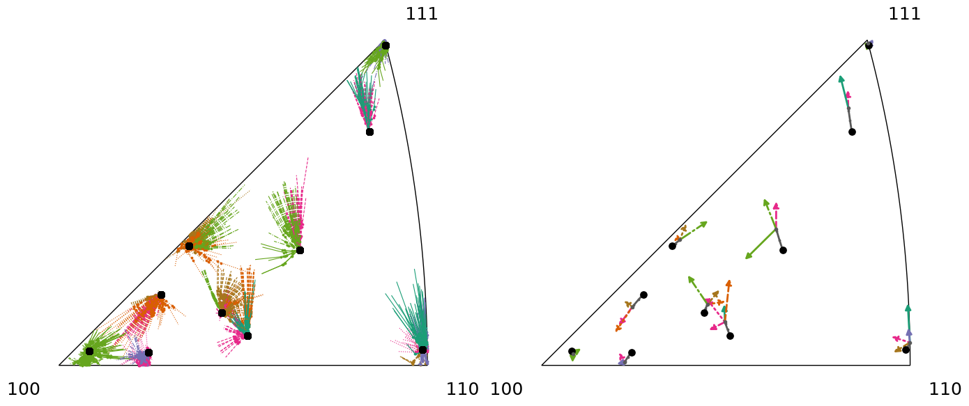
../_images/tutorials_reorientation-fragmentation_6_43.png

Reading the figure – visualizing fragmentation. The left panel is the evidence and the right panel is the interpretation. A grain whose elements stay in a tight bundle on the left is rotating almost rigidly (one fragment, one solid fork on the right); a grain whose elements fan out into two or more lobes is developing intragranular orientation gradients, and the segmenter turns each lobe into a distinctly colored + styled fork. Reading the two together tells you what kind of split it is: if the right panel forks but the left element clouds overlap in the IPF, the sub-grains are close in orientation and the split is more a spatial gradient than a sharp orientation bimodal (the graph segmenter uses spatial adjacency as well as orientation, so a grain’s sub-grains can share orientation yet occupy different regions). The number of forks is controlled by the segmenter (gamma for Leiden resolution, tol_deg for the misorientation edge cutoff); the left fan is the ground truth you calibrate those against. The per-grain fragment table (grain_id, n_fragments, fragment_sizes, n_elements) quantifies the right panel, and the fragments can be viewed in 3D in ParaView: IPFProcessor.add_element_field_to_exodus writes a per-element fragment_label scalar, and add_element_rgb_to_exodus writes a per-element RGB (rgb_x/y/z, mapped to color with scalar mapping off) in the same dark palette as this figure. For the colors to be meaningful, annotate the Exodus of the analyzed mesh (a co-registered loaded run’s mesh.e/sim_output.e beside the mesh_out you segmented) – the shipped bare cpfe_hex_fragmentation/mesh.e is a different microstructure, so the example colors it by block id only as a writer demo.

Why fragmentation matters. Intragranular fragmentation is not just descriptive: orientation gradients and nascent sub-boundaries are where geometrically necessary dislocations pile up, they are the precursors to recrystallization nuclei, and they frequently co-locate with damage initiation. Crucially, fragmentation is a distinct signal from stress or strain magnitude – a grain can be only moderately stressed yet fragment heavily (favourably oriented for multi-slip), or highly stressed yet rotate rigidly. That independence is exactly what makes “which grains fragment the most” worth flagging as a rare event in its own right.

From fragmentation to rare events (REI, and REI-vs-REI plots). Because fragmentation is an independent signal, it plugs into the same rare-event machinery used for stress or the Nye tensor, at two levels:

Grain level – rank grains by n_fragments (or fragment-size dispersion) and select the rare ones with rare_criteria_selection_library.select_highest_scalar, exactly the selector the REI pipeline uses for scalar fields. This is the capstone in section 4 below.
Field level – FragmentationAnalyzer().write_reorientation_field emits a per-element reorientation_deg scalar (misorientation from the reference step). Feed that CSV to IdentifyRareClusters with the abs_scalar_diff metric to find spatially coherent rare-reorientation clusters standalone, or combine reorientation_deg with nye_tensor_* / stress in a multi-feature SimilarityMetric so the clustering weighs fragmentation and mechanics together.

Both routes emit rare-cluster point clouds (VTK), so a fragmentation-driven REI can be overlaid against a stress- or GND-driven REI with REIComparison – the REI-vs-REI overlap plot (IoU/Dice, per-cluster matching) that answers “do the grains that fragment the most coincide with the grains that are most stressed?”. That comparison is the payoff of treating reorientation as a first-class REI criterion rather than a purely visual diagnostic.

3. Experiment: detect grain splits across load steps (FF / NF / EBSD)#

FragmentationAnalyzer().detect_splits finds one grain becoming several between two steps (cross-step graph + connected components). FF grain tables feed it directly; NF/EBSD reach the same detector via .segment (graph/Leiden) + .seg_to_grain_table. The shipped synthetic series has mixed multiplicity (1→1, 1→2, 1→3) with a ground_truth.json.

[4]:

import glob, json
gt = json.load(open("../../mwe_data/synthetic_split_ff/ground_truth.json"))
ff = sorted(glob.glob("../../mwe_data/synthetic_split_ff/ff_step*.csv"))
s = gt["split_step"]
res_ff = analyzer.detect_splits(ff[s - 1], ff[s], d_tol=20.0, theta_tol_deg=15.0, angle_type="degrees")
print(res_ff["n_splits"], res_ff["split_correspondences"])  # matches gt['n_splitting_grains']

3    parent_a children_b  n_children child_radii
0         2        2;6           2       10;10
1         3      3;7;8           3    10;10;10
2         5        5;9           2       10;10

4. Rare events: the grains that split the most#

Close the loop: rank grains by fragment count and flag the rare (most-fragmented) ones, reusing rare_criteria_selection_library.select_highest_scalar (the same REI selector used for nye/stress). Reorientation-from-initial (FragmentationAnalyzer().write_reorientation_field + the abs_scalar_diff metric) is the field-level analogue for full REI.

[5]:

from graintrace import rare_criteria_selection_library as rcs
rank = frags_df.rename(columns={"grain_id": "cluster_label", "n_elements": "n"})
rare = rcs.select_highest_scalar(rank, required_cols="n_fragments", k=3, min_size=1)
print("most-fragmented grains:", list(map(int, rare)))

most-fragmented grains: [4, 5, 6]

See :doc:/api/fragmentation, :doc:/api/ipf_orientation_tracking, and :doc:/api/plot_postprocessing for the API, and examples/demonstrate_reorientation_fragmentation.py for the full runnable script.