This tutorial is pure Python and runs from pip install graintrace — open it in Colab:

Rare-event identification on a 2D field

A minimal, self-contained rare-event identification (REI) run: build a small 2D von-Mises stress field with a few high-stress patches, cluster it with ClusterAnalysisIndicator, and visualize the field next to the recovered clusters. This tutorial is pure Python and runs from pip install graintrace.

See the algorithm page :doc:/algorithms/rare-event-identification and the API :class:~graintrace.ClusterAnalysisIndicator.

%matplotlib inline
import numpy as np
import pandas as pd
import matplotlib.pyplot as plt
from matplotlib.colors import ListedColormap, BoundaryNorm

from graintrace.cluster_indicator import ClusterAnalysisIndicator
from graintrace.similarity_metric_library import SimilarityMetricLibrary

Build a synthetic field

Each grid point gets a Cauchy-stress row (sxx..syz). The background is low stress; a handful of circular patches are raised to a high value, so the rare regions are known ahead of time.

def make_vms_grid(path, nx=30, ny=30, n_patches=10, vm_low=50.0, vm_high=200.0,
                  radius_range=(2, 5), seed=42):
    rng = np.random.default_rng(seed)
    vm = np.full((ny, nx), vm_low)
    for _ in range(n_patches):
        cx, cy = rng.integers(0, nx), rng.integers(0, ny)
        r = rng.integers(*radius_range)
        yy, xx = np.ogrid[:ny, :nx]
        vm[(xx - cx) ** 2 + (yy - cy) ** 2 <= r * r] = vm_high
    rows = []
    eid = 0
    for j in range(ny):
        for i in range(nx):
            eid += 1
            t = vm[j, i]
            rows.append(dict(id=eid, x=float(i), y=float(j), z=0.0,
                             sxx=t + rng.normal(0, t * 0.05),
                             syy=rng.normal(0, t * 0.02), szz=rng.normal(0, t * 0.02),
                             sxy=rng.normal(0, t * 0.02), sxz=rng.normal(0, t * 0.02),
                             syz=rng.normal(0, t * 0.02)))
    pd.DataFrame(rows).to_csv(path, index=False)
    return nx, ny

csv_path = "rei2d_field.csv"
nx, ny = make_vms_grid(csv_path)
print(f"wrote {csv_path}: {nx}x{ny} grid")

wrote rei2d_field.csv: 30x30 grid

Cluster with a von-Mises similarity metric

ClusterAnalysisIndicator runs a single-stage hierarchical clustering over a feature from a SimilarityMetricLibrary spec (here the von-Mises stress). threshold sets the distance cut of the dendrogram.

indicator = ClusterAnalysisIndicator(csv_path, coord_cols=("x", "y", "z"))
spec = SimilarityMetricLibrary().von_mises_stress()

run = indicator.run(
    method_type="scipy_hierarchical",
    spec=spec,
    threshold=0.01,
    method="average",
    criterion="distance",
)
result = run["points"]
print(result[["x", "y", "cluster_label"]].head())
print("n clusters:", result["cluster_label"].nunique())

/opt/hostedtoolcache/Python/3.11.17/x64/lib/python3.11/site-packages/sklearn/manifold/_mds.py:735: FutureWarning: The default value of `init` will change from 'random' to 'classical_mds' in 1.10. To suppress this warning, provide some value of `init`.
  warnings.warn(
/opt/hostedtoolcache/Python/3.11.17/x64/lib/python3.11/site-packages/sklearn/manifold/_mds.py:752: FutureWarning: The `dissimilarity` parameter is deprecated and will be removed in 1.10. Use `metric` instead.
  warnings.warn(

     x    y  cluster_label
0  0.0  0.0             16
1  1.0  0.0             16
2  2.0  0.0             20
3  3.0  0.0             17
4  4.0  0.0             20
n clusters: 22

Visualize field vs. clusters

def von_mises(df):
    s = {k: df[k].to_numpy() for k in ("sxx", "syy", "szz", "sxy", "sxz", "syz")}
    t1 = ((s["sxx"] - s["syy"]) ** 2 + (s["syy"] - s["szz"]) ** 2
          + (s["szz"] - s["sxx"]) ** 2) / 2.0
    t2 = 3.0 * (s["sxy"] ** 2 + s["sxz"] ** 2 + s["syz"] ** 2)
    return np.sqrt(t1 + t2)

vm_grid = von_mises(result).reshape(ny, nx)
labels = result["cluster_label"].to_numpy()
uniq = np.unique(labels)
idx = {lab: i for i, lab in enumerate(uniq)}
label_grid = np.vectorize(idx.get)(labels).reshape(ny, nx)
cmap = ListedColormap(plt.get_cmap("tab20")(np.linspace(0, 1, len(uniq))))
norm = BoundaryNorm(np.arange(len(uniq) + 1) - 0.5, len(uniq))

fig, ax = plt.subplots(1, 2, figsize=(9, 4))
im0 = ax[0].imshow(vm_grid, origin="lower", cmap="viridis")
ax[0].set_title("von-Mises stress")
fig.colorbar(im0, ax=ax[0], fraction=0.046, pad=0.04)
ax[1].imshow(label_grid, origin="lower", cmap=cmap, norm=norm)
ax[1].set_title(f"clusters (n={len(uniq)})")
plt.tight_layout()
plt.show()

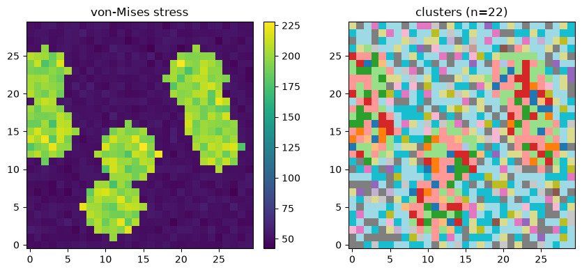
The high-stress patches come back as distinct clusters against the low-stress background.

See also

• Algorithm: :doc:/algorithms/rare-event-identification

• The full pipeline (graph clustering + hierarchical merge + rare-cluster export) in :doc:rare-event-identification

• 3D version: :doc:rei-example-3d