Rare-event identification (REI)#
A CPFE field has millions of numbers in it and a handful of places that matter. REI is the machinery for going from the first to the second: find the regions that are both extreme in a field and spatially coherent, and hand them back as labelled clusters you can export, count and compare.
The hard part is the word coherent. Thresholding a field gives you the extreme points, but they come back as speckle — isolated voxels scattered through the domain, most of them noise. What you actually want is a connected region that is extreme together. REI gets there in two stages:
Over-segment (
GraphSpatialCluster). Build a graph on the points, weight each edge by how similar its endpoints are in the chosen field, and run Leiden at a high resolution. This produces many small, internally uniform clusters. Spatial adjacency is baked into the graph, so a cluster is connected by construction.Merge in feature space (
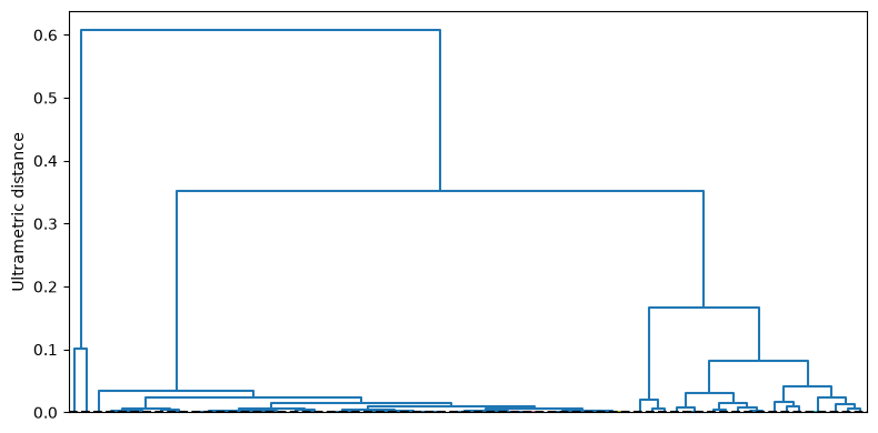
ClusterAnalysisIndicator). Reduce each stage-1 cluster to its mean feature vector and agglomerate hierarchically. Cutting that dendrogram atthresholdgroups clusters that are alike, whether or not they touch.
Then RareCriteria picks the rare ones out of the stage-2 result. Splitting it this way is what lets the two stages ask different questions — stage 1 is “is this one region?”, stage 2 is “is this region like that one?”.
Needs: pip install only (networkit Leiden, scipy hierarchical clustering, PyVista/VTK).
See the algorithm page Rare-event identification and the API IdentifyRareClusters.
Inputs#
A point-cloud CSV with an id column, x, y, z coordinates, and field columns. REI is not grid-locked: a regular grid uses the fast grid graph, arbitrary points fall back to the kNN graph. Two CPFE sources share the same schema:
mesh_out/out_element_centroid_*.csv: crisp per-element fields on the true mesh (mesh_csv="sync", the default), full fidelity, one row per element (kNN path). Preferred.grid_out/out_element_centroid_*.csv: a regular grid, fromgrid_transfer="per_step"or an offlineGridResampler(smoothed; see post-processing).
This notebook reads the shipped mwe_data/synthetic_vms.csv — a synthetic stress field with planted high-von-Mises regions — and writes everything it produces under out/rei/, leaving the sample data untouched.
Build the metric and the stage objects#
A SimilarityMetric is the pivot of the whole pipeline: it names the feature columns and a distance function over them, and that distance is what becomes the edge weight in stage 1. Here von_mises_stress() takes the six stress components and defines the distance between two points as the relative difference of their von Mises equivalent stress — so two points are “similar” when they are carrying a similar equivalent load, regardless of the stress state’s orientation.
Stage 2 needs its own metric over the reduced table, where every feature column has picked up a _mean suffix during the reduction. spec_reduced is the same distance function pointed at those renamed columns.
WeightConfig turns a distance into a weight. mode="rbf" gives \(w = \exp(-(d/\sigma)^{p})\), bounded in \((0, 1]\), which keeps the Leiden objective well conditioned; sigma_auto sets \(\sigma\) from a quantile of the sampled edge distances. (On near-identical orientation data sigma_auto collapses and shatters the segmentation — see segmentation — but on a smoothly varying stress field it is the right default.)
[1]:
import os

import numpy as np
import pandas as pd

from graintrace.rare_cluster_indicator import IdentifyRareClusters
from graintrace.similarity_metric_library import SimilarityMetricLibrary
from graintrace.user_data_class import SimilarityMetric, WeightConfig, RareCriteria
from graintrace import rare_criteria_selection_library as rcs

os.makedirs("out/rei", exist_ok=True)
filename = "../../mwe_data/synthetic_vms.csv"

metric_lib = SimilarityMetricLibrary()
spec = metric_lib.von_mises_stress()
spec_reduced = SimilarityMetric(
    name=spec.name + "_mean",
    feature_cols=[f"{c}_mean" for c in spec.feature_cols],
    func=spec.func,
)

weight_cfg = WeightConfig(
    mode="rbf",
    power=2.0,
    sigma=None,
    sigma_auto={"sample_size": 20_000, "random_state": 42, "quantile": 0.5},
)

print("stage-1 features:", spec.feature_cols)
print("stage-2 features:", spec_reduced.feature_cols)
print("points:", len(pd.read_csv(filename)))
stage-1 features: ['sxx', 'syy', 'szz', 'sxy', 'syz', 'sxz']
stage-2 features: ['sxx_mean', 'syy_mean', 'szz_mean', 'sxy_mean', 'syz_mean', 'sxz_mean']
points: 900
Run the two-stage clustering#
graph_mode="grid" builds the graph from grid adjacency within manhattan_radius (an \(\ell^1\) ball: radius 2 gives 12 neighbours on this \(30 \times 30\) 2D lattice, 24 in 3D), which is far cheaper than a kNN search when the points really are on a lattice. reduce_edges_topweights_k then keeps only each node’s 20 strongest edges.
networkit_kwargs["gamma"] is the Leiden resolution. High here — gamma=10.0 — because stage 1 is deliberately over-segmenting: it is better to cut a real region in half and let stage 2 glue it back together than to merge two unrelated regions that stage 2 can never separate again.
threshold=0.0005 cuts the stage-2 dendrogram with criterion="distance", so it is a distance in the metric’s units, not a cluster count. method="average" is UPGMA linkage. dendrogram_path writes the tree out so you can see where the cut lands rather than guessing the threshold.
[2]:
irc = IdentifyRareClusters(
    input_csv_path=filename, id_col="id", coord_cols=("x", "y", "z")
)
gsc, indicator = irc.make_stage_objects(graph_cluster_out="out/rei/reduced.csv")

bundle = irc.run_clustering(
    gsc=gsc,
    indicator=indicator,
    reduced_csv_path="out/rei/reduced.csv",
    gsc_run_kwargs=dict(
        spec=spec,
        graph_mode="grid",
        manhattan_radius=2,
        grid_tol=1e-6,
        n_jobs=1,
        weight_chunk_size=500_000,
        segmenter="leiden",
        seed=42,
        weight_cfg=weight_cfg,
        reduce_edges_topweights_k=20,
        networkit_kwargs={"gamma": 10.0},
        resume_from_checkpoint=False,
    ),
    indicator_run_kwargs=dict(
        method_type="scipy_hierarchical",
        spec=spec_reduced,
        threshold=0.0005,
        method="average",
        criterion="distance",
        dendrogram_path="out/rei/dendrogram.png",
    ),
)

print("stage-1 clusters:", len(np.unique(bundle["gsc_labels"])))
print("stage-2 clusters:", len(bundle["indicator_clusters_df"]))
Running clustering analysis...

=== Running GraphSpatialCluster ===

Data loaded.

Building graph with mode: grid
Building grid edges per node: 100%|██████████| 24/24 [00:00<00:00, 21779.16it/s]
Graph is built. Number of edges: 5102, Number of nodes: 900, Number of features: 6

Computing edge distances with metric: von_mises_stress
Edge distances: 100%|██████████| 5102/5102 [00:00<00:00, 12391047.49edge/s]
Estimated sigma for weight function: 0.03279019890086341

Converting edge distances to weights

Removing edges to keep only top 20 weights per node
Updated number of edges: 5102


Segmenting graph with method: leiden
Segmenter parameters: {'gamma': 10.0}
  NetworKit Leiden threads set to 1 (machine max 1)
Saved GSC labels: out/rei/reduced_gsc_labels.npy
Reduced CSV saved: out/rei/reduced.csv

Running cluster indicator

stage-1 clusters: 65
stage-2 clusters: 51
/opt/hostedtoolcache/Python/3.11.17/x64/lib/python3.11/site-packages/sklearn/manifold/_mds.py:735: FutureWarning: The default value of `init` will change from 'random' to 'classical_mds' in 1.10. To suppress this warning, provide some value of `init`.
  warnings.warn(
/opt/hostedtoolcache/Python/3.11.17/x64/lib/python3.11/site-packages/sklearn/manifold/_mds.py:752: FutureWarning: The `dissimilarity` parameter is deprecated and will be removed in 1.10. Use `metric` instead.
  warnings.warn(
The reduction is the whole point of the two-stage design: the stage-2 agglomeration runs on cluster means, not on every point, which is what makes hierarchical clustering tractable on a real field at all.
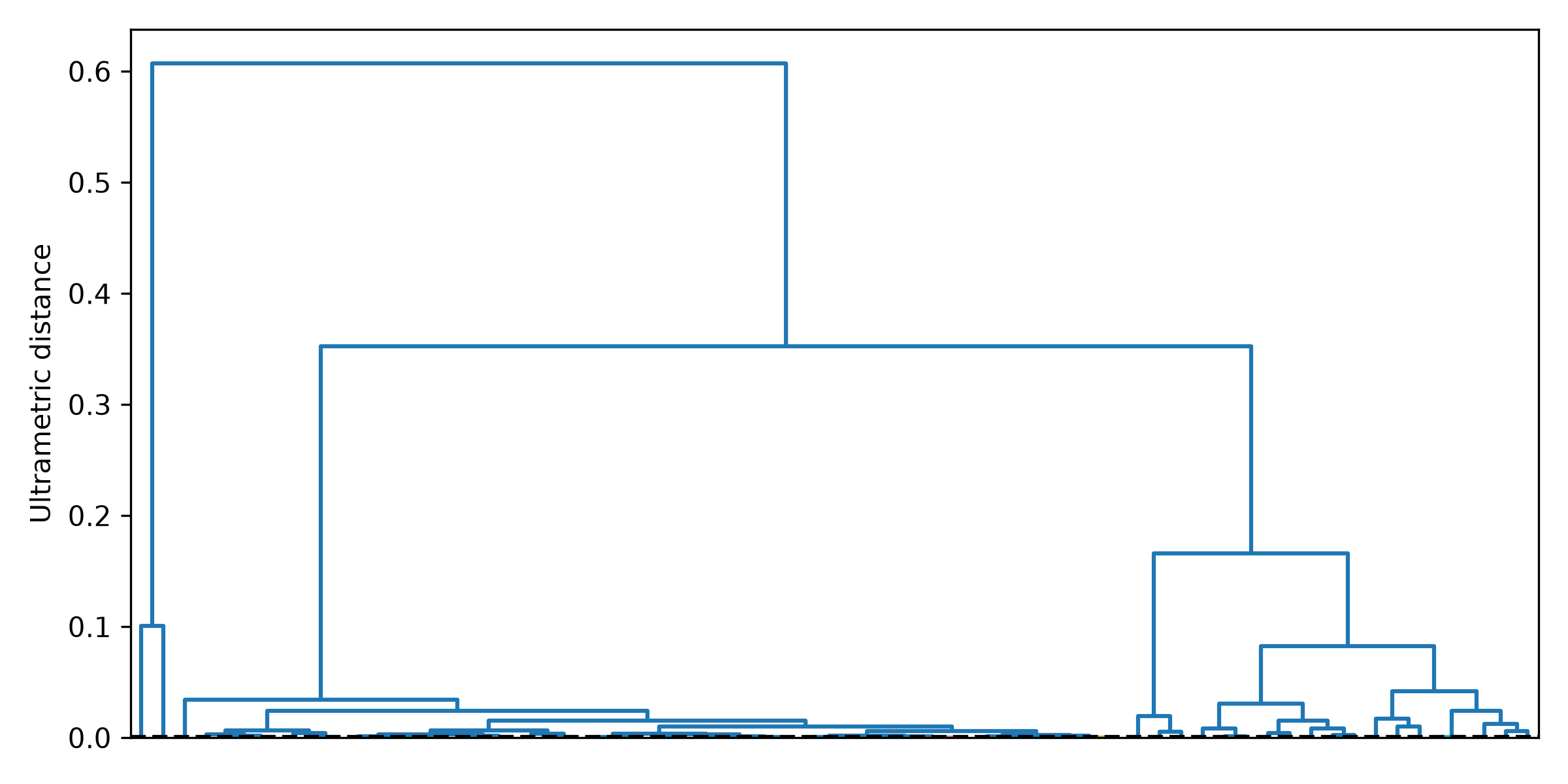
Read the counts honestly. 900 points became 65 stage-1 clusters, and threshold=0.0005 merged those into 51 — so most stage-1 clusters survived as singletons. That is a tight cut, and on this small synthetic field it is close to no merging at all. The dendrogram below is how you calibrate it: find the height at which the branches you consider “the same kind of region” join, and set threshold just above it. A larger threshold merges more aggressively and gives fewer, broader rare
regions.
[3]:
from IPython.display import Image

Image("out/rei/dendrogram.png")
[3]:
Select the rare clusters#
bundle["indicator_clusters_df"] carries one row per stage-2 cluster with cluster_label, the point count n, and min/max/sum/sumsq/mean for every coordinate and every reduced feature. Note the double suffix: the stage-1 reduction renamed szz to szz_mean, and the stage-2 aggregation then takes the mean of that, giving szz_mean_mean.
There is no ``von_mises_stress_mean_mean`` column — the aggregation is per-component, and von Mises is a nonlinear function of the components, so the pipeline cannot produce it by averaging. Derive it in the selector instead, which is exactly what RareCriteria is for: it takes any callable from the cluster table to a list of labels.
[4]:
print([c for c in bundle["indicator_clusters_df"].columns if c.endswith("_mean_mean")])
['sxx_mean_mean', 'syy_mean_mean', 'szz_mean_mean', 'sxy_mean_mean', 'sxz_mean_mean', 'syz_mean_mean']
[5]:
def highest_von_mises(df, k=3, min_size=1):
    """Rank stage-2 clusters by the von Mises stress of their mean stress tensor."""
    d = df.copy()
    s = {c: d[f"{c}_mean_mean"].to_numpy() for c in spec.feature_cols}
    d["von_mises_mean"] = np.sqrt(
        0.5
        * (
            (s["sxx"] - s["syy"]) ** 2
            + (s["syy"] - s["szz"]) ** 2
            + (s["szz"] - s["sxx"]) ** 2
        )
        + 3.0 * (s["sxy"] ** 2 + s["syz"] ** 2 + s["sxz"] ** 2)
    )
    return rcs.select_highest_scalar(
        d, k=k, required_cols="von_mises_mean", min_size=min_size
    )


rare_criteria = RareCriteria(selector=highest_von_mises)
print("rare labels:", highest_von_mises(bundle["indicator_clusters_df"]))
rare labels: [ 1 2 43]
Export#
run_get_rare_cluster applies the criteria and writes a VTK with the rare clusters as labelled blocks: background_block_id=1 for everything not selected, then first_rare_block_id=2 upward, one id per rare cluster. Open it in ParaView and threshold on the block id to see the rare regions in place.
rare_points_csv_path additionally writes the bare x, y, z, rare_cluster_id point cloud, which is the input format REI comparison expects — that is how you ask whether two different criteria flag the same places.
[6]:
out = irc.run_get_rare_cluster(
    bundle=bundle,
    criteria=rare_criteria,
    output_vtk_path="out/rei/rare_clusters.vtk",
    export_control="auto",
    background_block_id=1,
    first_rare_block_id=2,
    also_write_final_label=True,
    rare_reduced_stats_csv_path="out/rei/rare_cluster_stats.csv",
    rare_points_csv_path="out/rei/rare_points.csv",
)
print("VTK exported:", out["output_vtk_path"])

stats = pd.read_csv("out/rei/rare_cluster_stats.csv")
print(stats[["cluster_label", "n", "x_mean", "y_mean", "z_mean"]].to_string(index=False))
Saved rare cluster stats CSV: out/rei/rare_cluster_stats.csv

Saved rare point cloud CSV (51 points): out/rei/rare_points.csv
VTK exported: out/rei/rare_clusters.vtk
 cluster_label  n   x_mean   y_mean  z_mean
             1  1 0.087774 0.783699     0.0
             2  1 0.534483 0.931034     0.0
            43  1 0.219436 0.799373     0.0
Notes#
Checkpointing. Three restart levels exist for long runs: the bundle pickle, the reduced CSV plus the stage-1 labels array, and the graph edges themselves (
checkpoint_base_path+resume_from_checkpoint=True). The graph checkpoint deliberately does not comparesegmenteror the NetworKit options, so one checkpoint is reusable across a whole gamma sweep. See configuration.No multiprocessing. The pipeline is numba-threaded and single-process, so no
if __name__ == "__main__":guard is required — unlike NF reconstruction.``sigma_auto`` is field-dependent. Fine on a smooth stress field, actively harmful on orientation data where intra-grain edges are near-identical.
See also
Algorithm: Rare-event identification
Compare two REI outputs: REI comparison
Full script: examples/demonstrate_rei_pipeline.py