Post-CPFE analysis & plotting

A CPFE run leaves two very different kinds of output, and the first thing to get straight is which question each one answers.

The block CSV (out.csv) holds one row per time step and one column per grain per tensor component: cauchy_stress_xx_7 is the volume average of \(\sigma_{xx}\) over grain 7. It is small, it covers every step, and it is what you use for the macroscopic response and for per-grain time series.

The field directory (grid_out/, or mesh_out/) holds one CSV per written time step, with one row per spatial point and one column per tensor component. It is large, it exists only at the steps the run was told to write, and it is what you use for distributions, pole figures and rare-event identification.

SimulationResults wraps both behind one object so that a plotting call can ask for “ee at \(t = 1.0\)” without the caller knowing which file that lives in.

Needs: pip install only. The pole figure at the end additionally needs NEML2 v3 (neml2.texture).

The full script is examples/demonstrate_postprocess.py.

Inputs

The repo ships a complete 45-grain CPFE result under mwe_data/: out.csv for the block data and grid_out/ for the fields. FieldFileNaming tells SimulationResults how to recognise the per-step files and how to recover the step index from the filename — out_element_centroid_0024.csv is step 24 under the naming below.

If your own run produced no grid_out/ at all, that is the default: the CPFE driver only writes the regular grid every step when grid_transfer="per_step". Either rerun with that setting, use the per-element mesh_out/ CSVs (mesh_csv="sync", the default), or regenerate the grid offline from the Exodus with graintrace.grid_resampling.GridResampler. See the CPFE algorithm page for what each of those costs.

Load results

from graintrace.simulation_postprocessing import SimulationResults, FieldFileNaming
from graintrace import plot_postprocessing as postprocess

res = SimulationResults(
    block_csv="../../mwe_data/out.csv",
    field_dir="../../mwe_data/grid_out",
    field_naming=FieldFileNaming(
        prefix="out_element_centroid", index_width=4, sep="_", suffix=".csv"
    ),
)

print("block time steps :", res.n_steps)
print("grain ids        :", res.grain_ids)
print("field steps on disk:", sorted(res.field_files))
print("time of field steps:", [float(res.time[i]) for i in sorted(res.field_files)])

block time steps : 50
grain ids        : [1, 2, 3, 4, 5, 6, 7, 8, 9, 10, 11, 12, 13, 14, 15, 16, 17, 18, 19, 20, 21, 22, 23, 24, 25, 26, 27, 28, 29, 30, 31, 32, 33, 34, 35, 36, 37, 38, 39, 40, 41, 42, 43, 44, 45]
field steps on disk: [0, 4, 24, 49]
time of field steps: [0.0, 1.0, 1.21328125, 1.5140625]

Note the asymmetry that catches people out: there are 50 block time steps but only 4 field files. The block CSV is cheap enough to write every step; the field CSVs are not, so a run writes them at a handful of sync_times. Field step indices are the indices in ``res.field_files``, not positions in a list — here they are 0, 4, 24, 49, which are deliberately non-contiguous. Index into sorted(res.field_files) rather than assuming range(4).

Distributions at one time

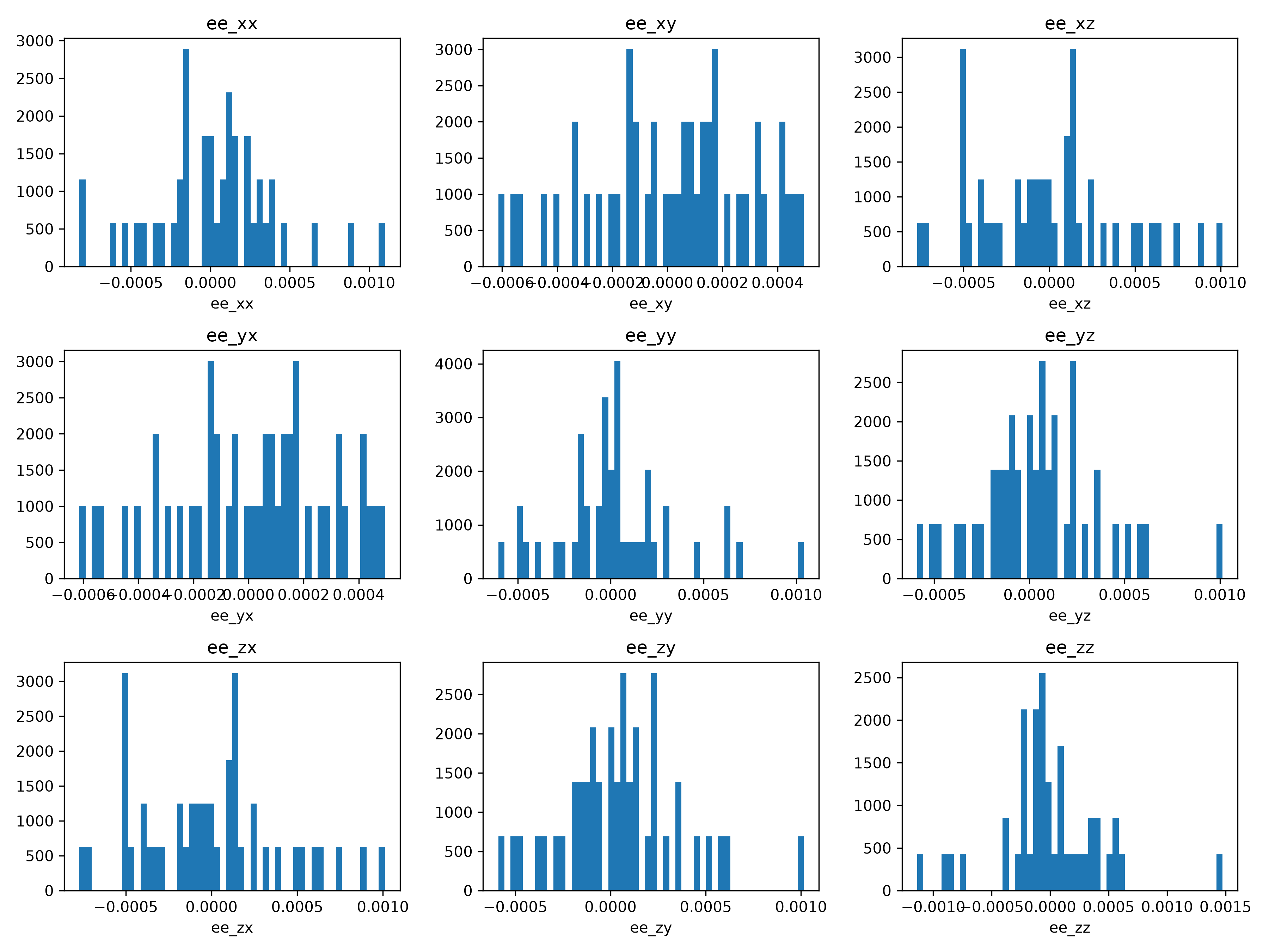
plot_block_properties_distribution takes a field at one time and plots the distribution of each component over all spatial points. tensor_prefix selects the field (ee, cauchy_stress, nye_tensor, ori_rodrigues, strain) and order is its tensor rank, which is what tells the plotter how many component columns to look for: order=2 means the six symmetric components xx, xy, xz, yy, yz, zz.

This is the plot that tells you whether a nominally uniform load is actually producing a uniform response. For a polycrystal it never is — grains with a soft slip system oriented for the load yield first, and the distribution develops the tail that rare-event identification goes looking for.

The plotters save to ``output_folder`` and do not call ``plt.show()``, so in a notebook you load the written PNG back to see it.

postprocess.plot_block_properties_distribution(
    res, time=1.0, tensor_prefix="ee", order=2, output_folder="out/post"
)
postprocess.plot_macroscopic_stress_strain(
    res,
    stress_tensor_prefix="cauchy_stress",
    strain_tensor_prefix="strain",
    volume_prefix="volume",
    output_folder="out/post",
)
postprocess.plot_block_properties_over_time(
    res, tensor_prefix="cauchy_stress", order=2, output_folder="out/post"
)

import os

print(sorted(os.listdir("out/post")))

['cauchy_stress_order2_over_time.png', 'ee_pdf_timeindex4.png', 'macro_stress_strain_cauchy_stress_vs_strain.png']

Elastic strain distribution

Each panel is one component of the elastic strain \(\varepsilon^{e}\) over the 12 000 grid points at \(t = 1.0\), which is the end of the load ramp-in and so very nearly the elastic state.

from IPython.display import Image

Image("out/post/ee_pdf_timeindex4.png")

Macroscopic stress-strain

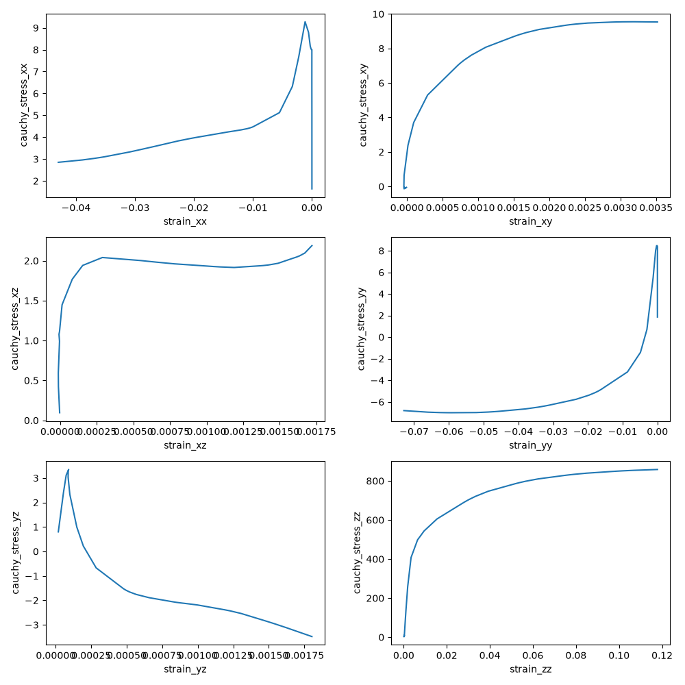
plot_macroscopic_stress_strain forms the volume-weighted average of stress and strain over all grains at every block time step,

\[\bar{\sigma} = \frac{\sum_g V_g \, \sigma_g}{\sum_g V_g}, \qquad \bar{\varepsilon} = \frac{\sum_g V_g \, \varepsilon_g}{\sum_g V_g},\]

and plots one component against the matching one. volume_prefix="volume" names the per-grain volume columns \(V_g\) that supply the weights; without them an unweighted mean would let a tiny grain count as much as a large one.

Read the zz panel: the load is prescribed along \(z\), and the curve shows the elastic rise and then the knee into plastic flow. The off-diagonal panels are the unconstrained response of an anisotropic aggregate — a uniaxial displacement on a polycrystal does not give a uniaxial stress state.

Image("out/post/macro_stress_strain_cauchy_stress_vs_strain.png")

Per-grain time series

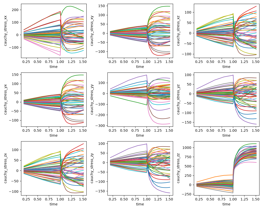
plot_block_properties_over_time plots one line per grain for each component, straight from the block CSV. This is the view that shows load partitioning: the spread between the lines at a given time is how differently oriented grains are carrying the same macroscopic load.

Image("out/post/cauchy_stress_order2_over_time.png")

Pole figures

plot_pole_figure reads the orientation field and projects it, so it answers a different question from the plots above: not how much load a grain carries, but which way its lattice points.

Two warnings about the inputs, both of which silently produce a wrong figure rather than an error:

• tensor_prefix="ori_rodrigues" is a misnomer. Those columns hold the NEML2 v3 modified Rodrigues parameters \(\tan(\theta/4)\,\hat{\mathbf{e}}\), not the classical Rodrigues-Gibbs vector \(\tan(\theta/2)\,\hat{\mathbf{e}}\). graintrace reads them correctly as MRP; a tool that assumes Rodrigues will not. See the notation page.

• crystal_symmetry must be the real point group. With "432" each orientation is folded over the 24 cubic rotations, so one grain contributes 24 poles.

direction=[0, 0, 1] requests the \(\{001\}\) family. construct_odf=False plots the discrete poles; True kernel-density-estimates an orientation distribution function first, which is what you want for many grains and misleading for ten.

postprocess.plot_pole_figure(
    res,
    tensor_prefix="ori_rodrigues",
    time=1.0,
    direction=[0, 0, 1],
    crystal_symmetry="432",
    device="cpu",
    output_folder="out/post",
    construct_odf=False,
)

print(sorted(f for f in os.listdir("out/post") if "figure" in f))

['inversepolefigure_discrete_001_timeindex4.png', 'polefigure_discrete_001_timeindex4.png']

Image("out/post/polefigure_discrete_001_timeindex4.png")

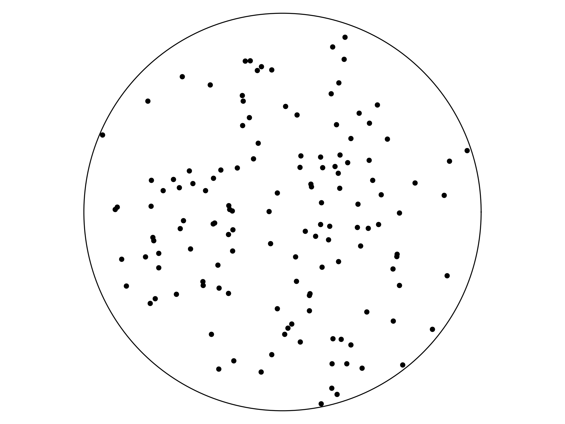
The same call also writes the inverse pole figure, which maps the sample \(z\) axis into the crystal’s standard stereographic triangle — the conventional way to read “which crystal direction is each grain presenting to the load”.

Gotchas

• Pre-load steps are near zero. Steps at or below initialize_time have near-zero stress and elastic strain by construction; that is the ramp-in, not a failed solve.

• Field indices are not positions. Use sorted(res.field_files); the step numbers are whatever the run wrote.

• ``out_element_centroid_0000.csv`` here is header-only. The shipped step-0 file has no data rows, because nothing had been written at \(t = 0\). Steps 24 and 49 carry the full 12 000 rows. A plotting call against step 0 gets an empty frame, not an error.

• Grid versus mesh fields. grid_out/ is a resampled regular grid; mesh_out/ is the true CPFE mesh, one row per element plus a block_id column giving the grain. Both work here. For anything extreme-sensitive prefer mesh_out/: resampling an Exodus smooths the grain-boundary extremes, because MOOSE stores the element fields as nodal projections.

• Experiments use a different loader. experiment_postprocessing.ExperimentResults has the same shape but its own FieldFileNaming (e.g. prefix expsyn_, suffix time.csv).

Where to go next

• Rare-event identification – find the rare regions in these fields.

• Reorientation & fragmentation – track how the orientations above move under load.

• the CPFE algorithm page – the constitutive model that produced the data.