Grinding example

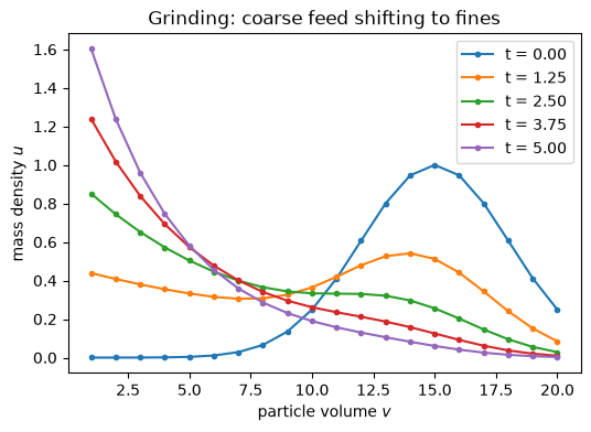
This notebook runs the fragmentation population balance model defined in grinding.i and plots the two things a grinding model is expected to show: the size distribution shifting from the coarse feed toward the fines, and conservation of total mass. The model, its math, and a walkthrough of the input file are described on the Population balance (fragmentation) page.

Breakage model

This example fixes the two constitutive choices (see Population balance (fragmentation) for the population balance equation and the flux operator derivation):

• Fragmentation rate – increasing with size, with a sink at the smallest bin, \(\gamma_i = 0.05\, i\) (so \(\gamma_0 = 0\)).

• Daughter distribution – each parent splits its mass equally over all smaller bins, \(p_{kj} = v_j / (j\, v_k)\) for \(k < j\), which conserves mass at uniform density.

%matplotlib inline
import matplotlib.pyplot as plt
import torch

import neml2

torch.set_default_dtype(torch.float64)

Load the input file, fetch the TransientDriver, and run the transient. driver.result() returns a flat dict of per step buffers keyed output.<step>.u.

factory = neml2.load_input("grinding.i")
driver = factory.get_driver("driver")
driver.run()
res = driver.result()

# Bin volumes and time axis match the [Tensors] block in grinding.i.
v = torch.arange(1.0, 21.0)
time = torch.linspace(0.0, 5.0, 25)
steps = sorted(int(k.split(".")[1]) for k in res if k.startswith("output.") and k.endswith(".u"))
u = torch.stack([res[f"output.{s}.u"].detach().reshape(-1) for s in steps])
u.shape

torch.Size([25, 20])

Size distribution evolution

The coarse Gaussian feed (centered at bin 14) breaks into smaller bins over time; mass accumulates in the low volume sink.

fig, ax = plt.subplots(figsize=(6, 4))
for s in [0, 6, 12, 18, 24]:
    ax.plot(v, u[s], marker="o", ms=3, label=f"t = {time[s]:.2f}")
ax.set_xlabel("particle volume $v$")
ax.set_ylabel("mass density $u$")
ax.set_title("Grinding: coarse feed shifting to fines")
ax.legend()
plt.show()

Mass conservation

The finite-volume flux form with zero-flux boundaries conserves total mass \(\sum_i u_i\,\Delta v_i\) (here \(\Delta v_i = 1\)) to solver tolerance at every step.

mass = u.sum(dim=1)
fig, ax = plt.subplots(figsize=(6, 4))
ax.plot(time, mass, marker="o", ms=3)
ax.set_xlabel("time")
ax.set_ylabel(r"total mass  $\sum_i u_i \Delta v_i$")
ax.set_title("Total mass is conserved")
ax.set_ylim(float(mass.min()) * 0.99, float(mass.max()) * 1.01)
plt.show()
print(f"relative mass drift: {(mass.max() - mass.min()) / mass[0]:.2e}")

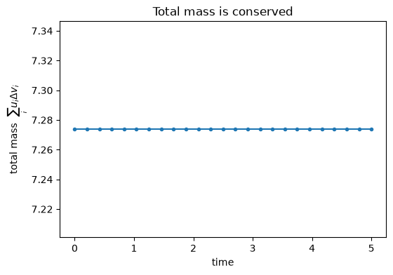
relative mass drift: 2.44e-16