Plotting pole figures

This example shows how to plot pole figures with the neml2.texture routines. It loads a crystal plasticity model, uses it to generate reorientation data under rolling, and then plots three kinds of texture figure: a discrete \(\{111\}\) pole figure, a discrete inverse pole figure, and a continuous \(\{111\}\) pole figure from a reconstructed orientation distribution function (ODF). Along the way it shows how to reconstruct a continuous ODF from discrete orientations, including cross-validated selection of the kernel half-width.

The model is the approximated single-crystal formulation in crystal_approximated.i (the same input used by the formulations example); it is integrated with pyzag. See the pyzag tutorial for more on the pyzag driver.

Note

This is a heavier example (500 crystals, 2500 time steps) and is committed pre-executed; it runs on the GPU when one is available.

Setup

This example simulates rolling in an FCC material: rate is the strain rate, total_rolling_strain the reduction strain, ntime the number of time steps, ncrystal the number of random initial orientations, and nchunk the pyzag time-integration chunk size.

import matplotlib.pyplot as plt
import torch

import neml2
from neml2.types import MRP, SR2, WR2, Scalar
import neml2.texture as texture
from pyzag import nonlinear, chunktime

torch.manual_seed(0)
torch.set_default_dtype(torch.double)
device = torch.device("cuda:0" if torch.cuda.is_available() else "cpu")
print(f"Using device: {device}")

nchunk = 20
ncrystal = 500

rate = 0.0001
total_rolling_strain = 0.5
ntime = 2500
end_time = total_rolling_strain / rate

Using device: cuda:0

The rolling history is the same isochoric stretch used in the formulations example: extension along \(y\), contraction along \(z\), no spin. The 500 initial orientations are sampled uniformly on \(SO(3)\) with MRP.rand.

deformation_rate = torch.zeros((ntime, ncrystal, 6), device=device)
deformation_rate[:, :, 1] = rate
deformation_rate[:, :, 2] = -rate
deformation_rate = SR2(deformation_rate)
vorticity = WR2(torch.zeros((ntime, ncrystal, 3), device=device))
times = torch.linspace(0, end_time, ntime, device=device).unsqueeze(-1).expand(ntime, ncrystal)

initial_orientations = MRP.rand(ncrystal, device=device)

Integrate the rolling deformation

The pyzag driver below packs the typed force tensors into the model’s flat force layout, seeds the initial orientation into the state vector, integrates the history, and slices the final orientation back out — the same metadata-safe round trip used in the formulations example.

def _state_layout(pmodel):
    for name in pmodel.slayout.vars():
        yield name, pmodel.slayout.var_size(name)


def integrate(pmodel, forces, seeds):
    # Pack the typed forces into the flat layout pyzag expects.
    forces = {name: forces[name] for name in pmodel.fvars}
    flat_forces = neml2.SparseVector(pmodel.flayout, forces).assemble().tensors[0].data

    # Initial state: zeros, with each seeded variable written into its slice.
    nstate = sum(size for _, size in _state_layout(pmodel))
    state0 = torch.zeros((ncrystal, nstate), device=device)
    offset = 0
    for name, size in _state_layout(pmodel):
        if name in seeds:
            state0[..., offset : offset + size] = seeds[name].reshape(ncrystal, size)
        offset += size

    solver = nonlinear.RecursiveNonlinearEquationSolver(
        pmodel,
        step_generator=nonlinear.StepGenerator(nchunk),
        predictor=nonlinear.PreviousStepsPredictor(),
        nonlinear_solver=chunktime.ChunkNewtonRaphson(rtol=1.0e-6, atol=1.0e-8),
    )
    return nonlinear.solve_adjoint(solver, state0, len(flat_forces), flat_forces)


def extract(pmodel, history, name):
    offset = 0
    for var, size in _state_layout(pmodel):
        if var == name:
            return history[..., offset : offset + size]
        offset += size
    raise KeyError(name)

nmodel = neml2.load_nonlinear_system("crystal_approximated.i", "eq_sys")
nmodel.to(device=device)
pmodel = neml2.pyzag.NEML2PyzagModel(nmodel)

with torch.no_grad():
    history = integrate(
        pmodel,
        {"t": Scalar(times, 0), "deformation_rate": deformation_rate, "vorticity": vorticity},
        {"orientation": initial_orientations.data},
    )

orientations = MRP(extract(pmodel, history, "orientation")[-1])
print("final orientations:", tuple(orientations.data.shape))

/tmp/ipykernel_2537202/356272241.py:20: UserWarning: pyzag lowered torch._functorch.config.donated_buffer's default to False process-wide. AOTAutograd 'donated buffers' (torch>=2.12) are incompatible with pyzag's retain_graph=True adjoint over torch.compile'd models, which otherwise raises 'compiled with non-empty donated buffers'. To keep donated buffers enabled, restore torch._functorch.config._config['donated_buffer'].default = True -- compiled models differentiated through the adjoint will then error.
  solver = nonlinear.RecursiveNonlinearEquationSolver(

final orientations: (500, 3)

Discrete pole figure

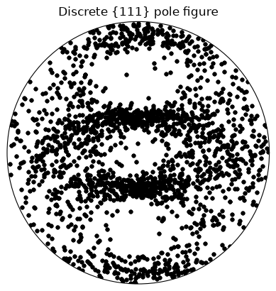
Plot a discrete \(\{111\}\) pole figure of the final orientations under cubic crystal symmetry ("432"). Each crystal contributes its symmetry-equivalent \(\{111\}\) poles projected onto the unit disk.

texture.pretty_plot_pole_figure_points(
    orientations, torch.tensor([1.0, 1.0, 1.0], device=device), crystal_symmetry="432"
)
plt.title("Discrete {111} pole figure")
plt.show()

Discrete inverse pole figure

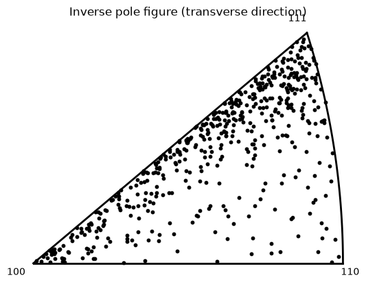
An inverse pole figure shows which crystal directions align with a chosen sample direction — here the transverse direction \([0, 1, 0]\).

texture.pretty_plot_inverse_pole_figure(
    orientations, torch.tensor([0.0, 1.0, 0.0], device=device), crystal_symmetry="432"
)
plt.title("Inverse pole figure (transverse direction)")
plt.show()

ODF reconstruction

Reconstruct a continuous ODF from the discrete orientations with a kernel density estimate. The de la Vallee Poussin kernel half-width is selected by cross-validation; we print the optimized value.

odf = texture.KDEODF(
    orientations, texture.DeLaValleePoussinKernel(torch.tensor(0.1, device=device))
)
odf.optimize_kernel()
print(f"optimized kernel half-width: {float(odf.kernel.h.detach()):.4f}")

optimized kernel half-width: 0.1837

Continuous pole figure

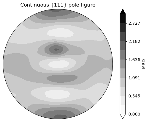
Use the reconstructed ODF to plot a smooth, continuous \(\{111\}\) pole figure. The contour values are in multiples of a random distribution (MRD).

texture.pretty_plot_pole_figure_odf(
    odf,
    torch.tensor([1.0, 1.0, 1.0], device=device),
    crystal_symmetry="432",
    limits=(0.0, 3.0),
    ncontour=12,
)
plt.title("Continuous {111} pole figure")
plt.show()