Transient driver

A TransientDriver walks a constitutive model through a prescribed load history, feeding each step’s converged state into the next step. In this tutorial you’ll ramp a strain from zero to 5% over 50 steps, run a perfect-viscoplastic model through that history, and plot the resulting stress–strain curve. The driver is configured from the same kind of input file you’ve been using.

The recursive update

Each step takes the previous state and the new forces and produces the next state:

for n in range(N):
    s[n + 1] = model(f[n + 1], s[n], f[n])

When NEML2 is coupled to an external PDE solver, that loop lives outside NEML2 — the host solver supplies the new forces and asks NEML2 for the new state. For self-contained workflows (verification, regression tests, parameter calibration, plotting a stress–strain curve), TransientDriver keeps everything inside NEML2.

Note

For training and adjoint-style sensitivities through a transient, prefer pyzag, which performs the same recursive update in a much more efficient fashion.

The input file

The [Drivers] block names the model to step, the prescribed time history, and the prescribed strain history. Time and the strain values are built inline in [Tensors]:

Listing 12 input.i

# Drive a perfect-viscoplastic constitutive model through a uniaxial
# strain history of 50 steps. The implicit-update model `model` is the
# same kind of object that previous tutorials evaluated point-wise —
# `TransientDriver` repeatedly calls it, threading converged state from
# step n into step n+1.

[Tensors]
  [times]
    type = Python
    expr = 'Scalar.linspace(0.0, 1.0, 50)'
  []
  [max_strain]
    type = Python
    expr = 'SR2.fill(0.05, -0.025, -0.025, 0.0, 0.0, 0.0)'
  []
  [strains]
    type = Python
    expr = 'SR2(torch.linspace(0.0, 1.0, 50, dtype=torch.float64).reshape(50, 1) * max_strain.data.unsqueeze(0))'
  []
[]

[Drivers]
  [driver]
    type = TransientDriver
    model = 'model'
    prescribed_time = 'times'
    force_SR2_names = 'E'
    force_SR2_values = 'strains'
  []
[]

[Models]
  [mandel_stress]
    type = IsotropicMandelStress
    cauchy_stress = 'stress'
  []
  [vonmises]
    type = SR2Invariant
    invariant_type = 'VONMISES'
    tensor = 'mandel_stress'
    invariant = 'effective_stress'
  []
  [yield_surface]
    type = YieldFunction
    yield_stress = 5
  []
  [flow]
    type = ComposedModel
    models = 'vonmises yield_surface'
  []
  [normality]
    type = Normality
    model = 'flow'
    function = 'yield_function'
    from = 'mandel_stress'
    to = 'flow_direction'
  []
  [flow_rate]
    type = PerzynaPlasticFlowRate
    reference_stress = 100
    exponent = 2
  []
  [Eprate]
    type = AssociativePlasticFlow
  []
  [Erate]
    type = SR2VariableRate
    variable = 'E'
  []
  [Eerate]
    type = SR2LinearCombination
    from = 'E_rate plastic_strain_rate'
    to = 'strain_rate'
    weights = '1 -1'
  []
  [elasticity]
    type = LinearIsotropicElasticity
    coefficients      = '1e5           0.3'
    coefficient_types = 'YOUNGS_MODULUS POISSONS_RATIO'
    rate_form = true
  []
  [integrate_stress]
    type = SR2BackwardEulerTimeIntegration
    variable = 'stress'
  []
  [implicit_rate]
    type = ComposedModel
    models = 'mandel_stress vonmises yield_surface normality flow_rate Eprate Erate Eerate elasticity integrate_stress'
  []
[]

[EquationSystems]
  [eq_sys]
    type = NonlinearSystem
    model = 'implicit_rate'
    unknowns = 'stress'
    residuals = 'stress_residual'
  []
[]

[Solvers]
  [newton]
    type = Newton
    linear_solver = 'lu'
  []
  [lu]
    type = DenseLU
  []
[]

[Models]
  [predictor]
    type = ConstantExtrapolationPredictor
    unknowns_SR2 = 'stress'
  []
  [model]
    type = ImplicitUpdate
    equation_system = 'eq_sys'
    solver = 'newton'
    predictor = 'predictor'
  []
[]

A few things worth pointing out:

• prescribed_time has shape (N,) — one time value per step. N sets the number of steps.

• The force_*_names / force_*_values pair wires a model input (here the strain E) to a tensor block that supplies its values at every step. Each force tensor must carry a leading axis of length N.

• Anything not listed as a prescribed force or initial condition starts at zero — so stress starts at zero at step 0.

The [Tensors] block builds a 50-step time vector \(t \in [0, 1]\) and a matching strain history that ramps linearly to a peak uniaxial strain of \(\varepsilon_{xx} = 5\%\) with lateral contractions consistent with isochoric deformation. See Cross-referencing for more examples of the type = Python block.

Building and running the driver

load_input(path).get_driver(name) builds the driver from the input file:

import neml2

factory = neml2.load_input("input.i")
driver = factory.get_driver("driver")
driver

<neml2.drivers.TransientDriver.TransientDriver at 0x7fd0972cb100>

The driver carries the parsed model, the prescribed-time tensor, and the prescribed forces. The number of steps comes from the leading axis of prescribed_time:

print("nsteps        =", driver.nsteps)
print("forces        =", list(driver.forces))
print("wrapped model =", type(driver.model).__name__)

nsteps        = 50
forces        = ['E']
wrapped model = ImplicitUpdate

driver.run() executes the time loop, threading each step’s converged state into the next step:

driver.run()

True

Reading the per-step output

driver.result() returns a flat dict keyed by input.<step>.<variable> and output.<step>.<variable>. Step 0 holds only the prescribed forces (the model isn’t called at step 0); every later step holds what the model returned:

results = driver.result()
print("total entries:", len(results))
print("step 0  keys:", [k for k in results if k.startswith("input.0.")])
print("step 1  inputs:", [k for k in results if k.startswith("input.1.")])
print("step 1  outputs:", [k for k in results if k.startswith("output.1.")])

total entries: 295
step 0  keys: ['input.0.t', 'input.0.E']
step 1  inputs: ['input.1.t', 'input.1.E', 'input.1.E~1', 'input.1.t~1']
step 1  outputs: ['output.1.stress']

(Aside on the ~k syntax: a variable name ending in ~k denotes its value from k steps back — E~1 is the previous step’s strain, t~1 the previous step’s time. The model sees both E and E~1 and computes a strain rate internally.)

Pulling per-step strain and stress out as 1-D tensors is a simple comprehension:

import torch

nsteps = driver.nsteps
times = torch.tensor([results[f"input.{i}.t"].item() for i in range(nsteps)])
strain_xx = torch.tensor(
    [results[f"input.{i}.E"][0].item() for i in range(nsteps)]
)
# Step 0 has no output -> stress is the zero initial condition.
stress_xx = torch.tensor(
    [0.0] + [results[f"output.{i}.stress"][0].item() for i in range(1, nsteps)]
)
print(f"max strain_xx = {strain_xx.max().item():.4f}")
print(f"max stress_xx = {stress_xx.max().item():.2f}")

max strain_xx = 0.0500
max stress_xx = 23.54

(Index [0] picks the first Mandel slot of the SR2 payload, which is the \(xx\) component.)

Plotting the stress–strain curve

With per-step strain_xx and stress_xx in hand, the curve is just a matplotlib call. matplotlib is available in the [dev] extras (pip install -e ".[dev]"):

import matplotlib.pyplot as plt

fig, ax = plt.subplots(figsize=(5, 4))
ax.plot(strain_xx, stress_xx, "C0o-", markersize=3)
ax.set_xlabel(r"$\varepsilon_{xx}$")
ax.set_ylabel(r"$\sigma_{xx}$")
ax.grid(True, alpha=0.3)
fig.tight_layout()

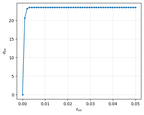
The initial linear segment is purely elastic. Once the von Mises stress exceeds the yield surface the Perzyna flow rule activates and the stress plateaus at the rate-dependent overstress level — a textbook perfect-viscoplastic response.

Saving the trajectory to disk

The full result dict can be saved to a single .pt file, keyed by the same strings driver.result() returns in memory:

driver.save_gold("result.pt")

loaded = torch.load("result.pt", weights_only=True)
print("entry count:", len(loaded))
print("a few keys :", list(loaded)[:4])

entry count: 295
a few keys : ['input.0.t', 'input.0.E', 'input.1.t', 'input.1.E']

This is the same format the regression suite’s TransientRegression consumes for its gold/result.pt references.

Where to go next

• To prescribe stress instead of strain, swap which variable the force_* block supplies; the rest of the workflow is unchanged.

• Give prescribed_time and the force tensors a trailing batch axis and the driver will sweep that axis in parallel — useful for parameter or initial-condition sweeps. See Vectorization for the batching rules.

• For gradient-based training through a transient response, see pyzag.