Composing with existing models

You’ll plug the ProjectileAcceleration model from the previous tutorials into a full trajectory simulation — alongside built-in time integrators, a Newton solve, and a transient driver — and let NEML2 wire everything up by matching variable names.

The full trajectory problem

A complete projectile trajectory model needs more than the acceleration formula. Let \(\boldsymbol{x}\) be the position and \(\boldsymbol{v}\) the velocity; the implicit time-integrated system is

(3)\[\begin{align} \dot{\boldsymbol{v}} & = \boldsymbol{a} = \boldsymbol{g} - \mu \boldsymbol{v}, \\ \mathbf{r}_{\boldsymbol{x}} &= \boldsymbol{x} - \boldsymbol{x}_n - (t - t_n)\,\dot{\boldsymbol{x}}, \\ \mathbf{r}_{\boldsymbol{v}} &= \boldsymbol{v} - \boldsymbol{v}_n - (t - t_n)\,\dot{\boldsymbol{v}}, \\ (\boldsymbol{x}, \boldsymbol{v}) &= \mathop{\mathrm{root}}_{\boldsymbol{x}, \boldsymbol{v}}\,\mathbf{r}. \end{align}\]

The four pieces map onto NEML2 building blocks as follows:

Equation	Building block
\(\dot{\boldsymbol{v}} = \boldsymbol{g} - \mu \boldsymbol{v}\)	The custom ProjectileAcceleration from the previous tutorials.
\(\dot{\boldsymbol{x}} = \boldsymbol{v}\) + the two backward-Euler residuals	Two VecBackwardEulerTimeIntegration instances, one per state variable.
root over \((\boldsymbol{x}, \boldsymbol{v})\)	An ImplicitUpdate wrapping the residual system.
Recursion through time	A TransientDriver sweeping a prescribed time array.

Each piece is its own block in [Models]; NEML2 connects them by matching output names to input names. The custom ProjectileAcceleration plugs in the same way a built-in would.

The input file

Listing 19 input.i

# Compose the custom ProjectileAcceleration with built-in time-integration
# and implicit-update blocks to integrate a projectile trajectory.

[Tensors]
  # Three different bags of balls, each bag a different drag coefficient.
  [mu]
    type = Python
    expr = 'Scalar(torch.tensor([0.1, 0.5, 1.0]))'
  []
  [times]
    type = Python
    expr = 'Scalar.linspace(0.0, 2.0, 100)'
  []
  # Initial conditions carry a TRAILING size-1 dynamic-batch placeholder
  # (-> shape (5, 1, *base)) so the (3,) viscosity broadcasts cleanly into
  # the second batch axis. The composed run evaluates 5 launches x 3
  # viscosities = 15 trajectories in one Newton solve per step.
  [x0]
    type = Python
    expr = 'Vec.zeros(5).dynamic_batch.unsqueeze(-1)'
  []
  [v0]
    type = Python
    expr = '''
      v0 = Vec.fill(6.0, 8.0, 0.0)
      v1 = Vec.fill(8.0, 7.0, 0.0)
      v2 = Vec.fill(10.0, 6.0, 0.0)
      v3 = Vec.fill(12.0, 5.0, 0.0)
      v4 = Vec.fill(14.0, 4.0, 0.0)
      stacked = stack([v0.dynamic_batch, v1.dynamic_batch, v2.dynamic_batch, v3.dynamic_batch, v4.dynamic_batch])
      result = stacked.dynamic_batch.unsqueeze(-1)
    '''
  []
[]

[Models]
  [eq1]
    type = ProjectileAcceleration
    velocity = 'v'
    acceleration = 'a'
    dynamic_viscosity = 'mu'
  []
  [eq2]
    type = VecBackwardEulerTimeIntegration
    variable = 'x'
    rate = 'v'
  []
  [eq3]
    type = VecBackwardEulerTimeIntegration
    variable = 'v'
    rate = 'a'
  []
  [residual]
    type = ComposedModel
    models = 'eq1 eq2 eq3'
  []
[]

[EquationSystems]
  [system]
    type = NonlinearSystem
    model = 'residual'
    unknowns = 'x v'
    residuals = 'x_residual v_residual'
  []
[]

[Solvers]
  [newton]
    type = Newton
    rel_tol = 1e-08
    abs_tol = 1e-10
    max_its = 50
    linear_solver = 'lu'
  []
  [lu]
    type = DenseLU
  []
[]

[Models]
  [eq4]
    type = ImplicitUpdate
    equation_system = 'system'
    solver = 'newton'
  []
[]

[Drivers]
  [driver]
    type = TransientDriver
    model = 'eq4'
    prescribed_time = 'times'
    ic_Vec_names = 'x v'
    ic_Vec_values = 'x0 v0'
  []
[]

A few things to notice in this file:

• ProjectileAcceleration sits next to the built-ins. The eq1 block uses our custom type just like eq2 / eq3 use the built-in VecBackwardEulerTimeIntegration.

• Wiring is implicit, through variable names. eq1 writes acceleration = 'a', and the velocity integrator eq3 reads rate = 'a'. Same story for v. NEML2 sees the matches and threads the values through, so a is not a free input of the composed residual.

• The rest of the blocks (residual, system, eq4, driver) bundle the three leaves into a single residual, declare which variables are unknowns, wrap the system in a Newton solve, and recurse it through time. See ComposedModel, ImplicitUpdate, and TransientDriver for the full option surface.

Inspecting the wiring

Before running anything, use neml2-inspect to print the resolved input/output graph of the composed residual block. Typos and forgotten renames show up here as unbound inputs or missing outputs, which is much easier to debug than a deep runtime traceback:

import sys, os
sys.path.insert(0, os.getcwd())

import projectile  # registers ProjectileAcceleration with the native factory

# `neml2-inspect` is the same CLI you'd call from the shell (with
# `--load projectile.py` to register the extension). We call the CLI's
# `main` in-process here so the same `import projectile` above does
# double duty and the output prints inline in the notebook.
from neml2.cli.inspect import main as _inspect_main
_inspect_main(["input.i", "residual"])

Model: ComposedModel

Inputs (6):
  v: type=Vec
  x: type=Vec
  x~1: type=Vec
  t: type=Scalar
  t~1: type=Scalar
  v~1: type=Vec

Outputs (2):
  x_residual: type=Vec
  v_residual: type=Vec

Parameters (1):
  eq1.mu: dtype=torch.float32, device=cpu, shape=[3]

Buffers (1):
  eq1.g: dtype=torch.float64, device=cpu, shape=[3]

0

The inputs are the trial state (x, v), the previous step’s state (x~1, v~1, t~1), and the new time t. Note that a does not appear — it’s resolved internally by eq1. The outputs are the two residuals x_residual and v_residual that the ImplicitUpdate will drive to zero.

Running the trajectory

The input file sets up a bag-of-balls scenario: three bags with different drag coefficients \(\mu\), each holding five balls thrown at different launch velocities. That’s 15 trajectories, all evaluated in a single batched Newton solve per step.

The batching falls out of broadcasting in [Tensors]: the launch velocity is a Vec whose dynamic-batch shape is (5, 1) (five launches, one placeholder viscosity slot), and mu is a Scalar with dynamic-batch shape (3,). When they meet inside eq1, the size-1 slot broadcasts against the three viscosities for a (5, 3) evaluation — one composed graph, one Newton iterate per step.

import neml2

factory = neml2.load_input("input.i")
driver = factory.get_driver("driver")
driver.run()

True

driver.result() returns a flat dict keyed by input.<step>.<var> / output.<step>.<var>. The leading (5, 3) on each step’s position and velocity is the batched (ball, bag) grid:

result = driver.result()
{k: tuple(v.shape) for k, v in result.items()
 if k.startswith("output.0.") or k.startswith("output.1.")}

{'output.1.x': (5, 3, 3), 'output.1.v': (5, 3, 3)}

Plotting the trajectories

Stack the per-step x outputs along a new leading time axis and project onto the \(x\)–\(y\) plane. One subplot per bag (viscosity), five trajectories each:

import torch
import matplotlib.pyplot as plt

nsteps = sum(1 for k in result if k.startswith("output.") and k.endswith(".x"))
positions = torch.stack(
    [result[f"output.{i}.x"] for i in range(1, nsteps + 1)]
).detach()  # shape (nsteps, 5 launches, 3 viscosities, 3 components)

mu_values = factory.get_tensor("mu").data.tolist()
n_launches = positions.shape[1]
n_visc = positions.shape[2]

fig, axes = plt.subplots(1, n_visc, figsize=(12, 4), sharey=True)
for k, ax in enumerate(axes):
    for j in range(n_launches):
        ax.plot(positions[:, j, k, 0], positions[:, j, k, 1], "-o", markersize=2,
                label=f"launch {j}")
    ax.set_xlabel("x")
    ax.set_title(rf"$\mu = {mu_values[k]:g}$")
    ax.set_xlim(-1, 26)
    ax.set_ylim(-12, 4)
    ax.axhline(0.0, color="black", linewidth=0.5)
    ax.grid(True)
axes[0].set_ylabel("y")
axes[-1].legend(loc="upper right", fontsize="small")
fig.tight_layout()
plt.show()

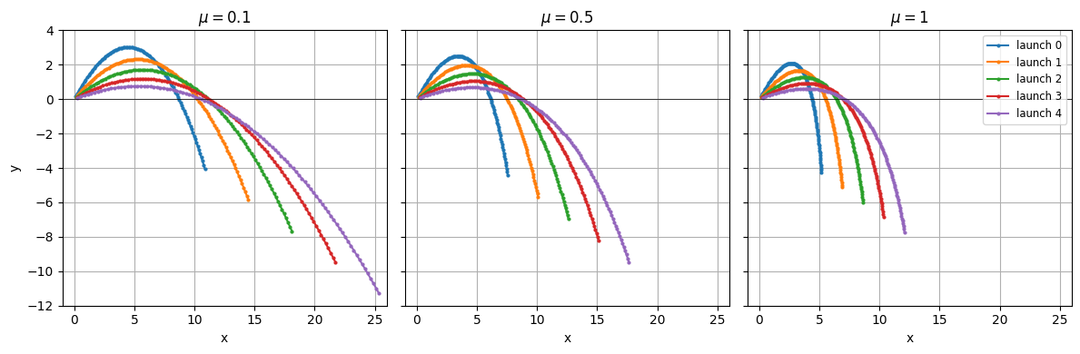
The lightly-damped bag (\(\mu = 0.1\)) sees the balls fly furthest; the heavily-damped bag (\(\mu = 1\)) drags them down within a few meters. All 15 trajectories ran in one Newton solve per step: the ProjectileAcceleration leaf is written in terms of a single (v, mu) pair, and the (5, 3) batch grid threads through every piece without any per-(launch, viscosity) bookkeeping in the leaf code.

Where to go next

• Model composition covers composition more broadly — the producer/consumer matching rules, multi-step chains, and parameter binding via output names.

• A composed model is itself a Model, so the same export, AOT-Inductor compilation, and outer composition paths apply to it — see Compiled models for the round trip.