Plotting polefigures

This example shows how to plot pole figures using the built-in neml2 postprocessing regimes. Specifically, this example load a crystal plasticity model, uses that model to generate reorientation data, and then plots two types of pole figures: discrete points and a contour plot from a reconstructed Orientation Distribution Function (ODF). In the process then this also demonstrates how to reconstruct a continuous ODF from discrete data.

Importing required libraries and setting up

This example will run on the GPU with CUDA if available. nchunk is the chunk size for the pyzag integration, ncrystal is the number of random initial crystal orientations to use.

This example simulates rolling in an FCC material. rate sets the strain rate, total_rolling_strain the reduction strain, and ntime the number of time steps to take.

import matplotlib.pyplot as plt
import torch
import neml2
import neml2.tensors
from pyzag import nonlinear, chunktime
import neml2.postprocessing

torch.set_default_dtype(torch.double)
if torch.cuda.is_available():
    dev = "cuda:0"
else:
    dev = "cpu"
device = torch.device(dev)
 
nchunk = 20
ncrystal = 500

rate = 0.0001
total_rolling_strain = 0.5
ntime = 2500
end_time = total_rolling_strain / rate
initial_orientations = neml2.Rot.rand((ncrystal,), ()).torch().to(device)

deformation_rate = torch.zeros((ntime, ncrystal, 6), device = device)
deformation_rate[:, :, 1] = rate
deformation_rate[:, :, 2] = -rate
times = torch.linspace(0, end_time, ntime, device = device).unsqueeze(-1).unsqueeze(-1).expand((ntime, ncrystal, 1))
vorticity = torch.zeros((ntime, ncrystal, 3), device = device)

pyzag driver

For more details on the pyzag driver used here see the deterministic and stochastic inference examples. This helper object just lets us integrate the crystal model using pyzag

class Solve(torch.nn.Module):
    """Just integrate the model through some strain history
 
    Args:
        discrete_equations: the pyzag wrapped model
        nchunk (int): number of vectorized time steps
        rtol (float): relative tolerance to use for Newton's method during time integration
        atol (float): absolute tolerance to use for Newton's method during time integration
    """
 
    def __init__(self, discrete_equations, nchunk=1, rtol=1.0e-6, atol=1.0e-8):
        super().__init__()
        self.discrete_equations = discrete_equations
        self.nchunk = nchunk
        self.rtol = rtol
        self.atol = atol
 
    def forward(self, time, deformation_rate, vorticity, cache=False, initial_orientations=None):
        """Integrate through some time/temperature/strain history and return stress
        Args:
            time (torch.tensor): batched times
            deformation_rate (torch.tensor): batched deformation rates
            vorticity (torch.tensor): batched vocticities
 
        Keyword Args:
            cache (bool): if true, cache the solution and use it as a predictor for the next call.
                This heuristic can speed things up during inference where the model is called repeatedly with similar parameter values.
        """
        solver = nonlinear.RecursiveNonlinearEquationSolver(
            self.discrete_equations,
            step_generator=nonlinear.StepGenerator(self.nchunk),
            predictor=nonlinear.PreviousStepsPredictor(),
            nonlinear_solver=chunktime.ChunkNewtonRaphson(rtol=self.rtol, atol=self.atol),
        )
 
        # Setup
        forces = {
            "forces/t": neml2.Scalar(time.squeeze(-1), 0),
            "forces/deformation_rate": neml2.SR2(deformation_rate, 0),
            "forces/vorticity": neml2.WR2(vorticity, 0),
            "forces/initial_orientation": neml2.Rot(initial_orientations, 0),
        }
        forces = [forces[key] for key in self.discrete_equations.fmap]
        forces = neml2.assemble_vector(forces, self.discrete_equations.flayout).torch()
        state0 = [neml2.Tensor()] * len(self.discrete_equations.smap)
        if initial_orientations is not None:
            i = self.discrete_equations.smap.index("state/orientation")
            state0[i] = neml2.Tensor(initial_orientations, 1)
        state0 = neml2.assemble_vector(state0, self.discrete_equations.slayout).torch()
 
        result = nonlinear.solve_adjoint(solver, state0, len(forces), forces)
 
        if cache:
            self.cached_solution = result.detach().clone()
 
        return result

Simulate rolling deformation

Simulate the rolling deformation and extract the final crystal orientations

nmodel = neml2.load_nonlinear_system("crystal.i", "eq_sys")
nmodel.to(device=device)
model = Solve(neml2.pyzag.NEML2PyzagModel(nmodel), nchunk=nchunk)

with torch.no_grad():
    orientations = neml2.tensors.Rot(
        model(times, deformation_rate, vorticity, initial_orientations=initial_orientations)[
            -1, :, 6:9
        ]
    )

Plot a discrete pole figure

Use the built-in routines to plot a discerete 111 pole figure of the final orientations.

neml2.postprocessing.pretty_plot_pole_figure_points(
    orientations, torch.tensor([1, 1, 1.0], device=device), crystal_symmetry="432"
)

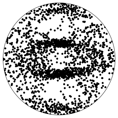
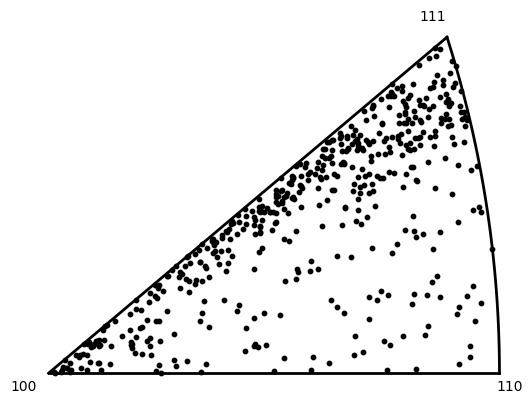
png

ODF reconstruction

Reconstruct the ODF from the discrete data. This example optimizes the kernel half-width with the build in routine (which uses a cross-validation approach). Print the final, optimal half width.

odf = neml2.postprocessing.odf.KDEODF(
    orientations, neml2.postprocessing.odf.DeLaValleePoussinKernel(torch.tensor(0.1))
)
odf.optimize_kernel(verbose=True)
print(odf.kernel.h)

loss: -1.34801e+00: 100%|██████████| 50/50 [00:38<00:00,  1.31it/s]

Parameter containing:
tensor(0.0712, requires_grad=True)

Plot a continuous polefigure

Use the reconstructed ODF to plot a continuous 111 polefigure

neml2.postprocessing.pretty_plot_pole_figure_odf(
    odf,
    torch.tensor([1, 1, 1.0], device=device),
    crystal_symmetry="432",
    limits=(0.0, 3.0),
    ncontour=12,
)

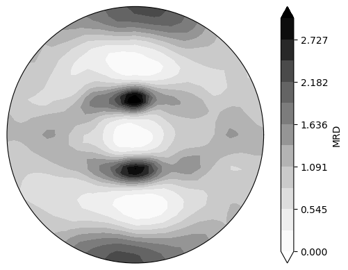
png