pyzag.nonlinear

Basic functionality for solving recursive nonlinear equations and calculating senstivities using the adjoint method

class pyzag.nonlinear.ExtrapolatingPredictor

Predict by extrapolating the values from the previous single steps

predict(results, k, kinc)

Predict the next steps

Parameters:

results (torch.tensor) – current results tensor, filled up to step k.
k (int) – start of current chunk
kinc (int) – next number of steps to predict

class pyzag.nonlinear.FullTrajectoryPredictor(history)

Predict steps using a complete user-provided trajectory

This is often used during optimization runs, where the provided trajectory could be the results from the previous step in the optimization routine

Parameters:: history (torch.tensor) – tensor of shape $(n_{time},...,n_{state})$ giving a complete previous trajectory

predict(results, k, kinc)

Predict the next steps

Parameters:

results (torch.tensor) – current results tensor, filled up to step k.
k (int) – start of current chunk
kinc (int) – next number of steps to predict

class pyzag.nonlinear.InitialOffsetStepGenerator(*args, initial_steps=None, **kwargs)

Generate chunks of recursive steps to produce at once

The user can provide a list of initial chunks to use, after which the object goes back to chunks of block_size

Parameters:

block_size (int) – regular chunk size
initial_steps (list of int) – initial steps

class pyzag.nonlinear.LastStepPredictor

Predict by providing the values from the previous single step

predict(results, k, kinc)

Predict the next steps

Parameters:

results (torch.tensor) – current results tensor, filled up to step k.
k (int) – start of current chunk
kinc (int) – next number of steps to predict

class pyzag.nonlinear.NonlinearRecursiveFunction(*args, **kwargs)

Basic structure of a nonlinear recursive function

This class has two basic responsibilities, to define the residual and Jacobian of the function itself and second to define the lookback.

The function and Jacobian are defined through forward so that this class is callable.

The lookback is defined as a property

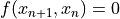
The function here defines a series through the recursive relation

$f(x_{n+1}, x_{n}, x_{n-1}, \ldots) = 0$

We denote the number of past entries in the time series used in defining this residual function as the lookback. A function with a lookback of 1 has the definition

$f(x_{n+1}, x_{n}) = 0$

A lookback of 2 is

$f(x_{n+1}, x_{n}, x_{n-1}) = 0$

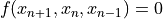
etc.

For the moment this class only supports functions with a lookback of 1!.

The function also must provide the Jacobian of the residual with respect to each input. So a function with lookback 1 must provide both

$J_{n+1} = \frac{\partial f}{\partial x_{n+1}}$

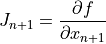
and

$J_{n} = \frac{\partial f}{\partial x_n}$

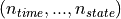
The input and output shapes of the function as dictated by the lookback and the desired amount of time-vectorization. Let’s call the number of time steps to be solved for at once $n_{block}$ and the lookback as $n_{lookback}$ . Let’s say our function has a state size $\left| x \right| = n_{state}$ . Our convention is the first dimension of input and output is the batch time axis and the last dimension is the true state size. The input shape of the state $x$ must be $(n_{block} + n_{lookback}, \ldots, n_{state})$ where $\ldots$ indicates some arbitrary number of batch dimensions. The output shape of the nonlinear residual will be $(n_{block}, \ldots, n_{state})$ . The output shape of the Jacobian will be $(n_{lookback} + 1, n_{block}, \ldots, n_{state}, n_{state})$ .

Additionally, we allow the function to take some driving forces as input. Mathematically we could envision these as an additional input tensor $u$ with shape $(n_{block} + n_{lookback}, \ldots, n_{force})$ and we expand the residual function definition to be

$f(x_{n+1}, x_{n}, x_{n-1}, \ldots, u_{n+1}, u_{n}, u_{n-1}, \ldots) = 0$

However, for convience we instead take these driving forces as python *args and **kwargs. Each entry in *args and **kwargs must have a shape of $(n_{block} + n_{lookback}, \ldots)$ and we leave it to the user to use each entry as they see fit.

To put it another way, the only hard requirement for driving forces is that the first dimension of the tensor must be slicable in the same way as the state $x$ .

class pyzag.nonlinear.Predictor: Base class for predictors

class pyzag.nonlinear.PreviousStepsPredictor

Predict by providing the values from the previous chunk of steps steps

predict(results, k, kinc)

Predict the next steps

Parameters:

results (torch.tensor) – current results tensor, filled up to step k.
k (int) – start of current chunk
kinc (int) – next number of steps to predict

class pyzag.nonlinear.RecursiveNonlinearEquationSolver(func, step_generator: ~pyzag.nonlinear.StepGenerator = <pyzag.nonlinear.StepGenerator object>, predictor: ~pyzag.nonlinear.Predictor = <pyzag.nonlinear.ZeroPredictor object>, direct_solve_operator: type[~pyzag.chunktime.BidiagonalOperator] = <class 'pyzag.chunktime.BidiagonalThomasFactorization'>, nonlinear_solver: ~pyzag.chunktime.NonlinearSolver = <pyzag.chunktime.ChunkNewtonRaphson object>, callbacks=None, convert_nan_gradients=True)

Generates a time series from a recursive nonlinear equation and (optionally) uses the adjoint method to provide derivatives

The series is generated in a batched manner, generating block_size steps at a time.

Parameters:

func (pyzag.nonlinear.NonlinearRecursiveFunction) – defines the nonlinear system

Keyword Arguments:

step_generator (pyzag.nonlinear.StepGenerator) – iterator to generate the blocks to integrate at once, default has a block size of 1 and no special fist step
predictor (pyzag.nonlinear.Predictor) – how to generate guesses for the nonlinear solve. Default uses all zeros
direct_solve_operator (pyzag.chunktime.LUFactorization) – how to solve the batched, blocked system of equations. Default is to use Thomas’s method
nonlinear_solver (pyzag.chunktime.ChunkNewtonRaphson) – how to solve the nonlinear system, default is plain Newton-Raphson
callbacks (None or list of functions) – callback functions to apply after a successful step
convert_nan_gradients (bool) – if True, convert NaN gradients to zero

accumulate(grad_result, full_adjoint, R, retain=False)

Accumulate the updated gradient values

Parameters:

grad_result (tuple of tensor) – current gradient results
full_adjoint (torch.tensor) – adjoint values
R (torch.tensor) – function values, for AD

Keyword Arguments:

retain (bool) – if True, retain the AD graph for a second pass

block_update(prev_solution, solution, forces)

Actually update the recursive system

Parameters:

prev_solution (tensor) – previous lookback steps of solution
solution (tensor) – guess at nchunk steps of solution
forces (list of tensors) – driving forces for next chunk plus lookback, to be passed as *args

block_update_adjoint(J, grads, a_prev)

Do the blocked adjoint solve

Parameters:

J (torch.tensor) – block of jacobians
grads (torch.tensor) – block of gradient values
a_prev (torch.tensor) – previous adjoint value

Returns:

next block of updated adjoint values

Return type:

adjoint_block (torch.tensor)

forward(*args, **kwargs)

Alias for solve

Parameters:

y0 (torch.tensor) – initial state values with shape (..., nstate)
n (int) – number of recursive time steps to solve, step 1 is y0
*args – driving forces to pass to the model

Keyword Arguments:

adjoint_params (None or list of parameters) – if provided, cache the information needed to run an adjoint pass over the parameters in the list

rewind(output_grad)

Rewind through an adjoint pass to provide the dot product for each quantity in output_grad

Parameters:: output_grad (torch.tensor) – thing to dot product with

solve(y0, n, *args, adjoint_params=None)

Solve the recursive equations for n steps

Parameters:

y0 (torch.tensor) – initial state values with shape (..., nstate)
n (int) – number of recursive time steps to solve, step 1 is y0
*args – driving forces to pass to the model

Keyword Arguments:

adjoint_params (None or list of parameters) – if provided, cache the information needed to run an adjoint pass over the parameters in the list

class pyzag.nonlinear.StepExtrapolatingPredictor

Predict by extrapolating using the previous chunks of steps

predict(results, k, kinc)

Predict the next steps

Parameters:

results (torch.tensor) – current results tensor, filled up to step k.
k (int) – start of current chunk
kinc (int) – next number of steps to predict

class pyzag.nonlinear.StepGenerator(block_size=1, first_block_size=0)

Generate chunks of recursive steps to produce at once

Parameters:

block_size (int) – regular chunk size
first_block_size (int) – if > 0 then use a special first chunk size, after that use block_size

reverse(): Reverse the iterator to yield chunks starting from the end

class pyzag.nonlinear.ZeroPredictor

Predict steps just using zeros

predict(results, k, kinc)

Predict the next steps

Parameters:

results (torch.tensor) – current results tensor, filled up to step k.
k (int) – start of current chunk
kinc (int) – next number of steps to predict

pyzag.nonlinear.solve(solver, y0, n, *forces)

Solve a pyzag.nonlinear.RecursiveNonlinearEquationSolver for a time history without the adjoint method

Parameters:

solver (py:class:pyzag.nonlinear.RecursiveNonlinearEquationSolver) – solve to apply
n (int) – number of recursive steps
*forces (*args of tensors) – driving forces

pyzag.nonlinear.solve_adjoint(solver, y0, n, *forces)

Apply a pyzag.nonlinear.RecursiveNonlinearEquationSolver to solve for a time history in an adjoint differentiable way

Parameters:

solver (pyzag.nonlinear.RecursiveNonlinearEquationSolver) – solve to apply
n (int) – number of recursive steps
*forces (*args of tensors) – driving forces