Deterministic material model calibration

This is a complete example of using the pyzag bindings to NEML2 to calibrate a material model against experimental data. demo_model.i defines the constitutive model, which is a structural material model describing the evolution of strain and stress in the material under mechanical load. The particular demonstration is a fairly complex model where the material responds differently as a function of both temperature and strain rate. The material deformation is driven by an axial strain and all the other stress components are zero.

In this example we:

1. Load the model in from an input file and wrap it for use in pyzag
2. Setup a grid of "experimental" conditions spanning several strain rates and temperatures
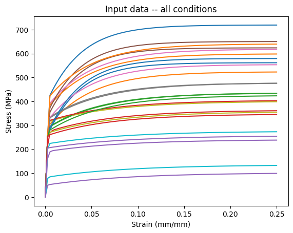
3. Replace the original model parameters with samples from a narrow normal distrubtion, centered on the orignial model mean, and run the model over the experimental conditions. This then becomes our synthetic input data.
4. Replace the original model parameters with random initial guesses (taken from a very wide normal distribution around the true values).
5. Setup the model calibration with a gradient-descent method by scaling the model parameters and resulting gradient values.
6. Calibrate the model against the synthetic experimental data.
7. Plot the results and print the calibrated parameter values, to see how close we can come to the true values.

The accuracy of the final model and the calibrated parameter values is heavily dependent on the choice of the normal distributions for the synthetic data and the initial parameter guesses. For narrow distributions for both the model can exactly recover the original parameter values. For wider distributions the calibrated model will not be exact, but will still accurately capture the mean of the synthetic tests.

import torch
import torch.distributions as dist
import neml2
from pyzag import nonlinear, reparametrization, chunktime
import matplotlib.pyplot as plt
from matplotlib.lines import Line2D
import tqdm

Setup parameters related to how we calibrate the model

Choose which device to use. The nchunk parameter controls the time integration in pyzag. pyzag can vectorize the time integration itself, providing a larger bandwidth to the compute device. This helps speed up the calculation, particularly when running on a GPU. The optimal value will depend on your compute device.

torch.manual_seed(0)
 
torch.set_default_dtype(torch.double)
if torch.cuda.is_available():
    dev = "cuda:0"
else:
    dev = "cpu"
device = torch.device(dev)
 
nchunk = 50

Setup the synthetic experimental conditions

Setup the loading conditions for the "experiments" we're going to run. These will span several strain rates (nrate) and temperatures (ntemperature). Overall, we'll run nbatch experiments. Also setup the maximum strain to pull the material through max_strain and the number of time steps we're going to use for integration ntime.

nrate = 5
ntemperature = 5
nbatch = nrate * ntemperature
max_strain = 0.25
ntime = 100
rates = torch.logspace(-6, 0, nrate, device=device)
temperatures = torch.linspace(310.0, 1190.0, ntemperature, device=device)

Define the variability in the synthetic data and for our initial guess at the parameters

These control the variability in the synthetic data (actual_cov) and the variability of the initial guess at the parameter values (guess_cov)

actual_cov = 0.025
guess_cov = 0.2

Setup the actual model

This class is a thin wrapper around the underlying pyzag wrapper for NEML2. All it does is take the input conditions (time, temperature, and strain), combine them into a single tensor, call the pyzag wrapper, and return the stress.

class SolveStrain(torch.nn.Module):
    """Just integrate the model through some strain history
 
    Args:
        discrete_equations: the pyzag wrapped model
        nchunk (int): number of vectorized time steps
        rtol (float): relative tolerance to use for Newton's method during time integration
        atol (float): absolute tolerance to use for Newton's method during time integration
    """
 
    def __init__(self, discrete_equations, nchunk=1, rtol=1.0e-6, atol=1.0e-4):
        super().__init__()
        self.discrete_equations = discrete_equations
        self.nchunk = nchunk
        self.cached_solution = None
        self.rtol = rtol
        self.atol = atol
 
    def forward(self, time, temperature, loading, cache=False):
        """Integrate through some time/temperature/strain history and return stress
        Args:
            time (torch.tensor): batched times
            temperature (torch.tensor): batched temperatures
            loading (torch.tensor): loading conditions, which are the input strain in the first base index and then the stress (zero) in the remainder
 
        Keyword Args:
            cache (bool): if true, cache the solution and use it as a predictor for the next call.
                This heuristic can speed things up during inference where the model is called repeatedly with similar parameter values.
        """
        if cache and self.cached_solution is not None:
            solver = nonlinear.RecursiveNonlinearEquationSolver(
                self.discrete_equations,
                step_generator=nonlinear.StepGenerator(self.nchunk),
                predictor=nonlinear.FullTrajectoryPredictor(self.cached_solution),
                nonlinear_solver=chunktime.ChunkNewtonRaphson(rtol=self.rtol, atol=self.atol),
            )
        else:
            solver = nonlinear.RecursiveNonlinearEquationSolver(
                self.discrete_equations,
                step_generator=nonlinear.StepGenerator(self.nchunk),
                predictor=nonlinear.PreviousStepsPredictor(),
                nonlinear_solver=chunktime.ChunkNewtonRaphson(rtol=self.rtol, atol=self.atol),
            )
 
        # We could pass this in as input, but it's easy enough to do here
        control = torch.zeros_like(loading)
        control[..., 1:] = 1.0
 
        # Setup
        forces = {
            "forces/t": neml2.Scalar(time, 0),
            "forces/T": neml2.Scalar(temperature, 0),
            "forces/fixed_values": neml2.SR2(loading, 0),
            "forces/control": neml2.SR2(control, 0),
        }
        forces = [forces[key] for key in self.discrete_equations.fmap]
        forces = neml2.assemble_vector(forces, self.discrete_equations.flayout).torch()
        state0 = torch.zeros(
            forces.shape[1:-1] + (self.discrete_equations.nstate,), device=forces.device
        )
 
        result = nonlinear.solve_adjoint(solver, state0, len(forces), forces)
 
        if cache:
            self.cached_solution = result.detach().clone()
 
        return result[..., 0:1]

Actually setup the model

Load the NEML model from disk, wrap it in both the pyzag wrapper and our thin wrapper class above. Exclude some of the model parameters we don't want to calibrate.

nmodel = neml2.load_nonlinear_system("demo_model.i", "eq_sys")
nmodel.to(device=device)
pmodel = neml2.pyzag.NEML2PyzagModel(
    nmodel,
    exclude_parameters=[
        "elasticity_E",
        "elasticity_nu",
        "R_X",
        "d_X",
        "mu_X",
        "mu_Y",
        "yield_zero_sy",
    ],
)
model = SolveStrain(pmodel)

Create the input tensors

Actually setup the full input tensors based on the parameters above

time = torch.zeros((ntime, nrate, ntemperature), device=device)
loading = torch.zeros((ntime, nrate, ntemperature, 6), device=device)
temperature = torch.zeros((ntime, nrate, ntemperature), device=device)
for i, rate in enumerate(rates):
    time[:, i] = torch.linspace(0, max_strain / rate, ntime, device=device)[:, None]
loading[..., 0] = torch.linspace(0, max_strain, ntime, device=device)[:, None, None]
for i, T in enumerate(temperatures):
    temperature[:, :, i] = T
time = time.reshape((ntime, -1))
temperature = temperature.reshape((ntime, -1))
loading = loading.reshape((ntime, -1, 6))

Replace the model parameters with random values

Sampled from a normal distribution controlled by the actual_cov parameter.

This controls the randomness in the input synthetic test data

# Replace with samples from normal
actual_parameter_values = {}
for n, p in model.named_parameters():
    actual_parameter_values[n] = p.data.detach().clone().cpu()
    ndist = dist.Normal(p.data, torch.abs(p.data) * actual_cov).expand((nbatch,) + p.shape)
    p.data = ndist.sample().to(device)

Run the model to generate the synthetic data

with torch.no_grad():
    data = model(time, temperature, loading)

Plot the synthetic data

plt.plot(loading.cpu()[..., 0], data[..., 0].cpu())
plt.xlabel("Strain (mm/mm)")
plt.ylabel("Stress (MPa)")
plt.title("Input data -- all conditions")
plt.show()

png

Setup the model for training

Replace the parameter values with random initial guesses, with variability controlled by the guess_cov parameter.

# Now replace our original parameter with random values over a range
guess_parameter_values = {}
for n, p in model.named_parameters():
    p.data = torch.normal(actual_parameter_values[n], torch.abs(actual_parameter_values[n])*guess_cov).to(device)
    guess_parameter_values[n] = p.data.detach().clone()

Scale the model parameters

Our material model parameters have units. In general, the parameter values will have different magnitudes from each other, which affects the scale of the gradients. Unbalanced gradients in turn affect the convergence of gradient descent optimization methods.

Typically we'd scale the training data to fix this problem. However, again our data has units and a physical meaning we want to preserve.

As an alternative we can scale the parameter values themselves both to clip the values to a physical range and to scale the gradients and hopefully improve the convergence of the optimization step. We do that here, in a way that should be mostly invisible to the training algorithms.

# Scale to get better performance
A_scaler = reparametrization.RangeRescale(
    torch.tensor(-12.0, device=device), torch.tensor(-4.0, device=device)
)
B_scaler = reparametrization.RangeRescale(
    torch.tensor(-1.0, device=device), torch.tensor(-0.5, device=device)
)
C_scaler = reparametrization.RangeRescale(
    torch.tensor(-8.0, device=device), torch.tensor(-3.0, device=device)
)
R_scaler = reparametrization.RangeRescale(
    torch.tensor([0.0, 0.0, 0.0, 0.0], device=device),
    torch.tensor([500.0, 500.0, 500.0, 500.0], device=device),
)
d_scaler = reparametrization.RangeRescale(
    torch.tensor([0.01, 0.01, 0.01, 0.01], device=device),
    torch.tensor([50.0, 50.0, 50.0, 50.0], device=device),
)
 
model_reparameterizer = reparametrization.Reparameterizer(
    {
        "discrete_equations.A_value": A_scaler,
        "discrete_equations.B_value": B_scaler,
        "discrete_equations.C_value": C_scaler,
        "discrete_equations.R_Y": R_scaler,
        "discrete_equations.d_Y": d_scaler,
    },
    error_not_provided=True,
)
model_reparameterizer(model)

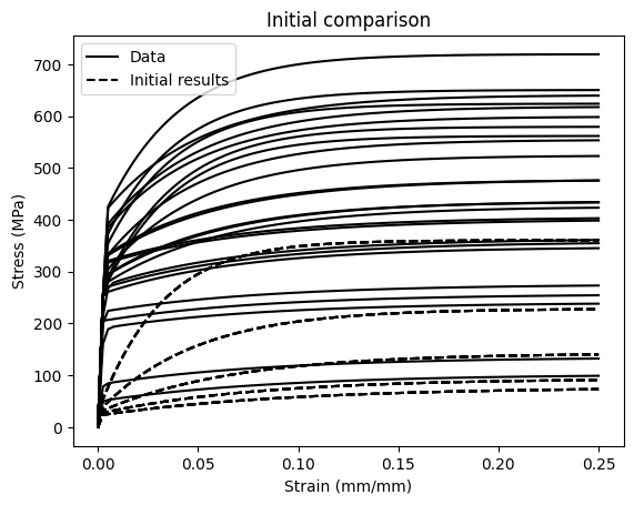
Run the model with the initial parameter values

Just to see how far away from the training data we starting from.

# Generate the initial results so we know where we are starting from
with torch.no_grad():
    initial_results = model(time, temperature, loading)

plt.plot(loading.cpu()[..., 0], data.cpu()[..., 0], "k-")
plt.plot(loading.cpu()[..., 0], initial_results.cpu()[..., 0], "k--")
plt.xlabel("Strain (mm/mm)")
plt.ylabel("Stress (MPa)")
plt.title("Initial comparison")
handles = [
    Line2D([], [], linestyle="-", color="k", label="Data"),
    Line2D([], [], linestyle="--", color="k", label="Initial results"),
]
plt.legend(handles=handles)
plt.show()

png

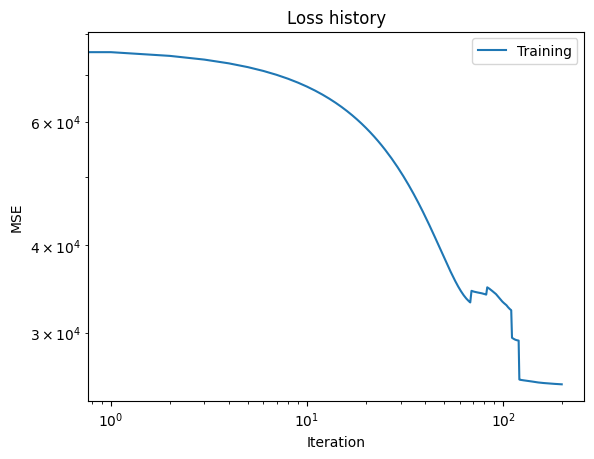
Calibrate the model against the synthetic data

Apply a fairly standard gradient-descent algorithm to adjust the model parameters to better match the synthetic data. Plot the loss versus iteration data from training.

niter = 200
lr = 5.0e-3
optimizer = torch.optim.Adam(model.parameters(), lr=lr)
loss_fn = torch.nn.MSELoss()
 
titer = tqdm.tqdm(
    range(niter),
    bar_format="{desc}{percentage:3.0f}%|{bar}|{n_fmt}/{total_fmt}{postfix}",
)
titer.set_description("Loss:")
loss_history = []
for i in titer:
    optimizer.zero_grad()
    res = model(time, temperature, loading, cache=True)
    loss = loss_fn(res, data)
    loss.backward()
    loss_history.append(loss.detach().clone().cpu())
    titer.set_description("Loss: %3.2e" % loss_history[-1])
    optimizer.step()
 
plt.loglog(loss_history, label="Training")
plt.xlabel("Iteration")
plt.ylabel("MSE")
plt.legend(loc="best")
plt.title("Loss history")
plt.show()

Loss: 2.53e+04: 100%|██████████|200/200

png

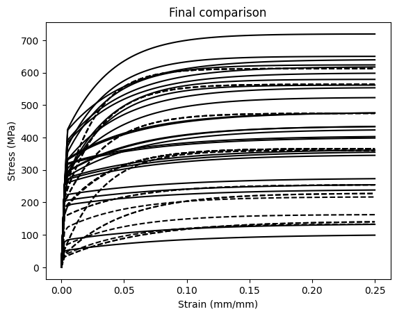
Plot the calibrated model predictions

See how accurately the calibrated model recovers the synthetic data.

plt.plot(loading.cpu()[..., 0], data.cpu()[...,0], "k-")
plt.plot(loading.cpu()[..., 0], res.detach().cpu()[...,0], "k--")
plt.xlabel("Strain (mm/mm)")
plt.ylabel("Stress (MPa)")
plt.title("Final comparison")
plt.show()

png

Print the calibrated model coefficients

These may vary sigifnicantly from the actual mean values, particularly if you used a large variance when sampling the parameters to generate the synthetic data.

print("The results:")
for n, p in model.discrete_equations.named_parameters():
    nice_name = n.split('.')[-2]
    ref_name = "discrete_equations." + nice_name
    scaler = model_reparameterizer.map_dict[ref_name]
    print(nice_name)
    print("\tInitial: \t" + str(guess_parameter_values[ref_name].cpu()))
    print("\tOptimized: \t" + str(scaler(p.data).cpu()))
    print("\tTrue value: \t" + str(actual_parameter_values[ref_name].cpu()))

The results:
A_value
    Initial:    tensor(-6.0041)
    Optimized:  tensor(-8.8544)
    True value:     tensor(-8.6790)
B_value
    Initial:    tensor(-0.7877)
    Optimized:  tensor(-0.9448)
    True value:     tensor(-0.7440)
C_value
    Initial:    tensor(-7.7675)
    Optimized:  tensor(-5.8379)
    True value:     tensor(-5.4100)
R_Y
    Initial:    tensor([334.1059, 156.6191,  72.0281,  54.0335])
    Optimized:  tensor([391.3497, 342.9169, 215.5262,  95.8719])
    True value:     tensor([300., 200., 100.,  50.])
d_Y
    Initial:    tensor([35.0282, 17.1230, 13.7900, 10.5681])
    Optimized:  tensor([43.9882, 34.7154, 30.0079, 19.7838])
    True value:     tensor([30., 20., 15., 12.])