Crystal plasticity formulations

There are two common ways to formulate crystal plasticity kinematics:

1. Integrate the elastic stretch and elastic rotation separately with two (coupled) rate equations.
2. Integrate the plastic deformation gradient $F_p$ directly from the plastic spatial velocity gradient $l_p$.

Both formulations are based on the usual multiplicative decomposition of the deformation gradient into elastic and plastic parts $F = F_e F_p$. This notebook calls the first approach the "separated" method and the second the "integrated" method (because the first splits the kinematics into two coupled equations and the second integrates a single equation for $F_p$).

It's easy to formulate a crystal model either way in NEML2 reusing most of detailed constitutive model objects like the hardening law, the slip law, and the crystal geometry. In fact the vast majority of the objects are shared between the two models with only a few specialized submodels required for each.

This example runs equivalent separated and integrated models through the same deformation history (rolling to 50% rolling strain) and plots a comparison. You can also use this notebook to look at differences in performance, though we have not done detailed performance optimization on either.

Importing required libraries and setting up

This example will run on the GPU with CUDA if available. nchunk is the chunk size for the pyzag integration, ncrystal is the number of random initial crystal orientations to use.

This example simulates rolling in an FCC material. rate sets the strain rate, total_rolling_strain the reduction strain, and ntime the number of time steps to take.

We need to calculate both the deformation rate/vorticity and the deformation gradient

import matplotlib.pyplot as plt
from matplotlib.lines import Line2D
import torch
import neml2
import neml2.tensors
from pyzag import nonlinear, chunktime
import neml2.postprocessing

torch.set_default_dtype(torch.double)
if torch.cuda.is_available():
    dev = "cuda:0"
else:
    dev = "cpu"
device = torch.device(dev)
 
nchunk = 10
ncrystal = 500

rate = 0.0001
total_rolling_strain = 0.5
ntime = 2500
end_time = total_rolling_strain / rate
initial_orientations = neml2.tensors.Rot.rand((ncrystal,), ()).torch().to(device)

deformation_rate = torch.zeros((ntime, ncrystal, 6), device=device)
deformation_rate[:, :, 1] = rate
deformation_rate[:, :, 2] = -rate
times = (
    torch.linspace(0, end_time, ntime, device=device)
    .unsqueeze(-1)
    .unsqueeze(-1)
    .expand((ntime, ncrystal, 1))
)
vorticity = torch.zeros((ntime, ncrystal, 3), device=device)

# Now get the integrated deformation gradient
full_spatial_velocity_gradient = (
    neml2.tensors.R2(neml2.tensors.SR2(deformation_rate)).torch()
    + neml2.tensors.R2(neml2.tensors.WR2(vorticity)).torch()
)
F = torch.zeros_like(full_spatial_velocity_gradient)
F[0] = torch.eye(3, device=device)
dt = torch.diff(times, dim=0)
Finc = torch.linalg.matrix_exp(full_spatial_velocity_gradient[:-1] * dt.unsqueeze(-1))
for i in range(1, ntime):
    F[i] = Finc[i - 1] @ F[i - 1]

pyzag driver for the separated model

For more details on the pyzag driver used here see the deterministic and stochastic inference examples. This helper object just lets us integrate the crystal model using pyzag

class SolveSeparate(torch.nn.Module):
    """Just integrate the model through some strain history
 
    Args:
        discrete_equations: the pyzag wrapped model
        nchunk (int): number of vectorized time steps
        rtol (float): relative tolerance to use for Newton's method during time integration
        atol (float): absolute tolerance to use for Newton's method during time integration
    """
 
    def __init__(self, discrete_equations, nchunk=1, rtol=1.0e-6, atol=1.0e-8):
        super().__init__()
        self.discrete_equations = discrete_equations
        self.nchunk = nchunk
        self.rtol = rtol
        self.atol = atol
 
    def forward(self, time, deformation_rate, vorticity, initial_orientations=None):
        """Integrate through some time/temperature/strain history and return stress
        Args:
            time (torch.tensor): batched times
            deformation_rate (torch.tensor): batched deformation rates
            vorticity (torch.tensor): batched vocticities
 
        Keyword Args:
            initial_orientation (torch.tensor): if provided, the initial orientations for each crystal
        """
        solver = nonlinear.RecursiveNonlinearEquationSolver(
            self.discrete_equations,
            step_generator=nonlinear.StepGenerator(self.nchunk),
            predictor=nonlinear.PreviousStepsPredictor(),
            nonlinear_solver=chunktime.ChunkNewtonRaphson(rtol=self.rtol, atol=self.atol),
        )
 
        # Setup
        forces = {
            "forces/t": neml2.Scalar(time.squeeze(-1), 0),
            "forces/deformation_rate": neml2.SR2(deformation_rate, 0),
            "forces/vorticity": neml2.WR2(vorticity, 0),
            "forces/initial_orientation": neml2.Rot(initial_orientations, 0),
        }
        forces = [forces[key] for key in self.discrete_equations.fmap]
        forces = neml2.assemble_vector(forces, self.discrete_equations.flayout).torch()
        state0 = [neml2.Tensor()] * len(self.discrete_equations.smap)
        if initial_orientations is not None:
            i = self.discrete_equations.smap.index("state/orientation")
            state0[i] = neml2.Tensor(initial_orientations, 1)
        state0 = neml2.assemble_vector(state0, self.discrete_equations.slayout).torch()
 
        result = nonlinear.solve_adjoint(solver, state0, len(forces), forces)
 
        return result

Simulate rolling deformation for the seperated model

Simulate the rolling deformation and extract the final crystal orientations

nmodel_separate = neml2.load_nonlinear_system("crystal.i", "eq_sys")
nmodel_separate.to(device = device)
model_separate = SolveSeparate(neml2.pyzag.NEML2PyzagModel(nmodel_separate), nchunk = nchunk)

with torch.no_grad():
    results_seperate = model_separate(times, deformation_rate, vorticity, initial_orientations = initial_orientations)
orientations_separate = neml2.tensors.Rot(results_seperate[-1,:,6:9])

ODF reconstruction for the seperated model

Reconstruct the ODF from the discrete data. Uncommenting the two lines will optimize the kernel half-width with the built in routine (which uses a cross-validation approach). However, for consistency between the two methods, we'll use a fixed half width for both.

odf_separate = neml2.postprocessing.odf.KDEODF(
    orientations_separate, neml2.postprocessing.odf.DeLaValleePoussinKernel(torch.tensor(0.2))
)
odf_separate.optimize_kernel(verbose = True)
print(odf_separate.kernel.h)

loss: -4.78125e-01: 100%|██████████| 50/50 [00:36<00:00,  1.36it/s]

Parameter containing:
tensor(0.2319, requires_grad=True)

pyzag driver for the integrated model

Same thing as for the separated model, just now for the integrated form where we take the deformation gradient as input. Don't forget to set the initial plastic deformation gradient to the identity!

class SolveIntegrated(torch.nn.Module):
    """Just integrate the model through some strain history
 
    Args:
        discrete_equations: the pyzag wrapped model
        nchunk (int): number of vectorized time steps
        rtol (float): relative tolerance to use for Newton's method during time integration
        atol (float): absolute tolerance to use for Newton's method during time integration
    """
 
    def __init__(self, discrete_equations, nchunk=1, rtol=1.0e-6, atol=1.0e-8):
        super().__init__()
        self.discrete_equations = discrete_equations
        self.nchunk = nchunk
        self.rtol = rtol
        self.atol = atol
 
    def forward(self, time, deformation_gradient, initial_orientations=None):
        """Integrate through some time/temperature/strain history and return stress
        Args:
            time (torch.tensor): batched times
            deformation_gradient (torch.tensor): batched deformation gradients
 
        Keyword Args:
            initial_orientation (torch.tensor): if provided, the initial orientations for each crystal
        """
        solver = nonlinear.RecursiveNonlinearEquationSolver(
            self.discrete_equations,
            step_generator=nonlinear.StepGenerator(self.nchunk),
            predictor=nonlinear.PreviousStepsPredictor(),
            nonlinear_solver=chunktime.ChunkNewtonRaphson(rtol=self.rtol, atol=self.atol),
        )
 
        # Setup
        forces = {
            "forces/t": neml2.Scalar(time.squeeze(-1), 0),
            "forces/F": neml2.R2(deformation_gradient, 0),
            "forces/r": neml2.Rot(initial_orientations, 0),
        }
        forces = [forces[key] for key in self.discrete_equations.fmap]
        forces = neml2.assemble_vector(forces, self.discrete_equations.flayout).torch()
        state0 = [neml2.Tensor()] * len(self.discrete_equations.smap)
        i = self.discrete_equations.smap.index("state/Fp")
        state0[i] = neml2.tensors.Tensor(
            torch.eye(3, device=time.device).unsqueeze(0).expand(time.shape[1:2] + (3, 3)), 1
        )
        state0 = neml2.assemble_vector(state0, self.discrete_equations.slayout).torch()
 
        result = nonlinear.solve_adjoint(solver, state0, len(forces), forces)
 
        return result

Simulate for the multiplicative model

Again, simulate rolling deformation

nmodel_integrated = neml2.load_nonlinear_system("crystal_integrated.i", "eq_sys")
nmodel_integrated.to(device=device)
model_integrated = SolveIntegrated(neml2.pyzag.NEML2PyzagModel(nmodel_integrated), nchunk=nchunk)

with torch.no_grad():
    results_integrated = model_integrated(times, F, initial_orientations=initial_orientations)
end_results_integrated = results_integrated[-1]

Extract the orientations for the multiplicative model

This takes some doing. We first need to get $F_p$ from the state, then calculate $F_e = F F_p^{-1}$, then do a polar decomposition to get the rotation as a matrix, then convert to modified Rodrigues parameters. Finally compose with the original texture to get the final, deformed texture.

split_state = neml2.disassemble_vector(
    neml2.Tensor(end_results_integrated, 1), model_integrated.discrete_equations.slayout
)
iFp = model_integrated.discrete_equations.smap.index("state/Fp")
Fp = split_state[iFp].torch().reshape(-1, 3, 3)
Flast = F[-1]
Fe = Flast @ torch.linalg.inv(Fp)
U, S, Vh = torch.linalg.svd(Fe)
Re = U @ Vh
Ue = Vh.transpose(-2, -1).conj() @ torch.diag_embed(S, dim1=-2, dim2=-1) @ Vh
Re_mrp = neml2.tensors.Rot.fill_matrix(neml2.tensors.R2(Re))
 
Q0 = neml2.tensors.Rot(initial_orientations)
Q = Re_mrp * Q0

Construct the ODF for the multiplicative model results

Basically the same as for the separated approach.

odf_integrated = neml2.postprocessing.odf.KDEODF(
    Q, neml2.postprocessing.odf.DeLaValleePoussinKernel(torch.tensor(0.2))
)
odf_integrated.optimize_kernel(verbose = True)
print(odf_integrated.kernel.h)

loss: -4.78211e-01: 100%|██████████| 50/50 [00:36<00:00,  1.35it/s]

Parameter containing:
tensor(0.2318, requires_grad=True)

Plot the pole figures

Use the reconstructed ODFs to plot continuous 111 polefigure

neml2.postprocessing.pretty_plot_pole_figure_odf(
    odf_separate,
    torch.tensor([1, 1, 1.0], device=device),
    crystal_symmetry="432",
    limits=(0.0, 3.0),
    ncontour=12,
)
neml2.postprocessing.pretty_plot_pole_figure_odf(
    odf_integrated,
    torch.tensor([1, 1, 1.0], device=device),
    crystal_symmetry="432",
    limits=(0.0, 3.0),
    ncontour=12,
)

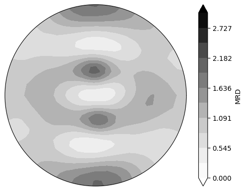
png

png

Plot some comparisons of the elastic strains

Extract the elastic strains from each model and plot:

1. The history of each crystal over time
2. The average over time

The averages are consistent but there are some differences in stress/elastic strain history between crystals when calculated this way.

state_history_split = neml2.disassemble_vector(
    neml2.Tensor(results_seperate, 2), model_separate.discrete_equations.slayout
)
state_history_mult = neml2.disassemble_vector(
    neml2.Tensor(results_integrated, 2), model_integrated.discrete_equations.slayout
)
 
iFp = model_integrated.discrete_equations.smap.index("state/Fp")
Fp_mult = state_history_mult[iFp].torch().reshape(F.shape[:-2] + (3, 3))
Fe_mult = F @ torch.linalg.inv(Fp_mult)
U_mult, S_mult, Vh_mult = torch.linalg.svd(Fe_mult)
Re_mult = U_mult @ Vh_mult
Ue_mult = Vh_mult.transpose(-2, -1).conj() @ torch.diag_embed(S_mult, dim1=-2, dim2=-1) @ Vh_mult
E_mult = 0.5 * (Ue_mult.transpose(-2, -1) @ Ue_mult - torch.eye(3, device=device))
ie = model_separate.discrete_equations.smap.index("state/elastic_strain")
 
plt.plot(times[:, 0, 0].cpu(), state_history_split[ie].torch()[:, :, 2].cpu(), "k-", alpha=0.5)
plt.plot(times[:, 0, 0].cpu(), E_mult[:, :, 2, 2].cpu(), "r--", alpha=0.5)
plt.xlabel("Time")
plt.ylabel("Elastic strain in the rolling direction")
plt.legend(
    [
        Line2D([0], [0], color="k", alpha=0.5),
        Line2D([0], [0], color="r", alpha=0.5, linestyle="--"),
    ],
    ["Seperate", "Integrated"],
    loc="best",
)

<matplotlib.legend.Legend at 0x7506a84e67b0>

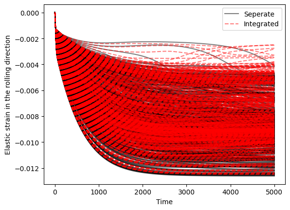
png

for i in range(3):
    plt.plot(
        times[:, 0, 0].cpu(),
        torch.mean(state_history_split[ie].torch()[:, :, i], dim=-1).cpu(),
        "k-",
        alpha=0.5,
    )
    plt.plot(times[:, 0, 0].cpu(), torch.mean(E_mult[:, :, i, i], dim=-1).cpu(), "r--", alpha=0.5)
plt.xlabel("Time")
plt.ylabel("Elastic strain")
plt.legend(
    [
        Line2D([0], [0], color="k", alpha=0.5),
        Line2D([0], [0], color="r", alpha=0.5, linestyle="--"),
    ],
    ["Seperate", "Integrated"],
    loc="best",
)

<matplotlib.legend.Legend at 0x75050b0b1810>

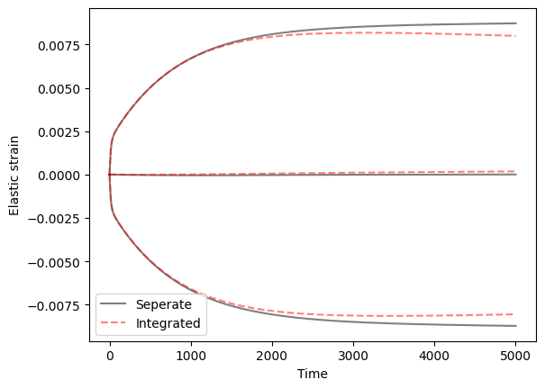
png