Transient driver#

A TransientDriver walks a constitutive model through a prescribed load history, feeding each step’s converged state into the next step. In this tutorial we’ll ramp a strain from zero to 5% over 50 steps, run a perfect-viscoplastic model through that history, and plot the resulting stress–strain curve. The driver is configured from the same kind of input file we’ve been using.

The recursive update#

Each step takes the previous state s and the new prescribed variables g (the given values) and produces the next state:

for n in range(N):
    s[n + 1] = model(g[n + 1], s[n], g[n])

When NEML2 is coupled to an external PDE solver, that loop lives outside NEML2 — the host solver supplies the new prescribed variables and asks NEML2 for the new state. For self-contained workflows like parameter calibration or plotting a stress–strain curve, TransientDriver keeps everything inside NEML2.

Note

For training and adjoint-style sensitivities through a transient, prefer pyzag, which performs the same recursive update in a much more efficient fashion.

The input file#

The [Drivers] block names the model to step, the prescribed time history, and the prescribed strain history. Time and the strain values are built inline in [Tensors]:

%%writefile input.i
# Drive a perfect-viscoplastic constitutive model through a uniaxial
# strain history of 50 steps. The implicit-update model `model` is the
# same kind of object that previous tutorials evaluated point-wise —
# `TransientDriver` repeatedly calls it, threading converged state from
# step n into step n+1.

[Tensors]
  [times]
    type = Python
    expr = 'linspace(Scalar(0.0).dynamic_batch, Scalar(1.0).dynamic_batch, 50)'
  []
  [max_strain]
    type = Python
    expr = 'SR2.fill(0.05, -0.025, -0.025, 0.0, 0.0, 0.0)'
  []
  [strains]
    type = Python
    expr = 'SR2(torch.linspace(0.0, 1.0, 50, dtype=torch.float64).reshape(50, 1) * max_strain.data.unsqueeze(0))'
  []
[]

[Drivers]
  [driver]
    type = TransientDriver
    model = 'model'
    prescribed_time = 'times'
    prescribed_SR2_names = 'E'
    prescribed_SR2_values = 'strains'
  []
[]

[Models]
  [mandel_stress]
    type = IsotropicMandelStress
    cauchy_stress = 'stress'
  []
  [vonmises]
    type = SR2Invariant
    invariant_type = 'VONMISES'
    tensor = 'mandel_stress'
    invariant = 'effective_stress'
  []
  [yield_surface]
    type = YieldFunction
    yield_stress = 5
  []
  [flow]
    type = ComposedModel
    models = 'vonmises yield_surface'
  []
  [normality]
    type = Normality
    model = 'flow'
    function = 'yield_function'
    from = 'mandel_stress'
    to = 'flow_direction'
  []
  [flow_rate]
    type = PerzynaPlasticFlowRate
    reference_stress = 100
    exponent = 2
  []
  [Eprate]
    type = AssociativePlasticFlow
  []
  [Erate]
    type = SR2VariableRate
    variable = 'E'
  []
  [Eerate]
    type = SR2LinearCombination
    from = 'E_rate plastic_strain_rate'
    to = 'strain_rate'
    weights = '1 -1'
  []
  [elasticity]
    type = LinearIsotropicElasticity
    coefficients      = '1e5           0.3'
    coefficient_types = 'YOUNGS_MODULUS POISSONS_RATIO'
    rate_form = true
  []
  [integrate_stress]
    type = SR2BackwardEulerTimeIntegration
    variable = 'stress'
  []
  [implicit_rate]
    type = ComposedModel
    models = 'mandel_stress vonmises yield_surface normality flow_rate Eprate Erate Eerate elasticity integrate_stress'
  []
[]

[EquationSystems]
  [eq_sys]
    type = NonlinearSystem
    model = 'implicit_rate'
    unknowns = 'stress'
    residuals = 'stress_residual'
  []
[]

[Solvers]
  [newton]
    type = Newton
    linear_solver = 'lu'
  []
  [lu]
    type = DenseLU
  []
[]

[Models]
  [predictor]
    type = ConstantExtrapolationPredictor
    unknowns_SR2 = 'stress'
  []
  [model]
    type = ImplicitUpdate
    equation_system = 'eq_sys'
    solver = 'newton'
    predictor = 'predictor'
  []
[]

Writing input.i

A few things worth pointing out:

prescribed_time has shape (N,) — one time value per step. N sets the number of steps.
The prescribed_*_names / prescribed_*_values pair wires a model input (here the strain E) to a tensor block that supplies its values at every step. Each prescribed tensor must carry a leading axis of length N.
Anything not listed as a prescribed variable or initial condition starts at zero — so stress starts at zero at step 0.

The [Tensors] block builds a 50-step time vector \(t \in [0, 1]\) and a matching strain history that ramps linearly to a peak uniaxial strain of \(\varepsilon_{xx} = 5\%\) with lateral contractions consistent with isochoric deformation. See Cross-referencing for more examples of the type = Python block.

Building and running the driver#

load_input(path).get_driver(name) builds the driver from the input file:

import neml2

factory = neml2.load_input("input.i")
driver = factory.get_driver("driver")
driver

<neml2.drivers.TransientDriver.TransientDriver at 0x7ff525b56380>

The driver carries the parsed model, the prescribed-time tensor, and the prescribed variables. The number of steps comes from the leading axis of prescribed_time:

print("nsteps        =", driver.nsteps)
print("prescribed    =", list(driver.prescribed))
print("wrapped model =", type(driver.model).__name__)

nsteps        = 50
prescribed    = ['E']
wrapped model = ImplicitUpdate

driver.run() executes the time loop, threading each step’s converged state into the next step:

driver.run()

True

Reading the per-step output#

driver.result() returns a flat dict keyed by input.<step>.<variable> and output.<step>.<variable>. Step 0 holds only the prescribed variables (the model isn’t called at step 0); every later step holds what the model returned:

results = driver.result()
print("total entries:", len(results))
print("step 0  keys:", [k for k in results if k.startswith("input.0.")])
print("step 1  inputs:", [k for k in results if k.startswith("input.1.")])
print("step 1  outputs:", [k for k in results if k.startswith("output.1.")])

total entries: 295
step 0  keys: ['input.0.t', 'input.0.E']
step 1  inputs: ['input.1.t', 'input.1.E', 'input.1.E~1', 'input.1.t~1']
step 1  outputs: ['output.1.stress']

(Aside on the ~k syntax: a variable name ending in ~k denotes its value from k steps back — E~1 is the previous step’s strain, t~1 the previous step’s time. The model sees both E and E~1 and computes a strain rate internally.)

Pulling per-step strain and stress out as 1-D tensors is a simple comprehension:

import torch

nsteps = driver.nsteps
times = torch.tensor([results[f"input.{i}.t"].item() for i in range(nsteps)])
strain_xx = torch.tensor([results[f"input.{i}.E"][0].item() for i in range(nsteps)])
# Step 0 has no output -> stress is the zero initial condition.
stress_xx = torch.tensor(
    [0.0] + [results[f"output.{i}.stress"][0].item() for i in range(1, nsteps)]
)
print(f"max strain_xx = {strain_xx.max().item():.4f}")
print(f"max stress_xx = {stress_xx.max().item():.2f}")

max strain_xx = 0.0500
max stress_xx = 23.54

(Index [0] picks the first Mandel slot of the SR2 payload, which is the \(xx\) component.)

Plotting the stress–strain curve#

With per-step strain_xx and stress_xx in hand, the curve is just a matplotlib call. matplotlib is available in the [dev] extras (pip install -e ".[dev]"):

import matplotlib.pyplot as plt

fig, ax = plt.subplots(figsize=(5, 4))
ax.plot(strain_xx, stress_xx, "C0o-", markersize=3)
ax.set_xlabel(r"$\varepsilon_{xx}$")
ax.set_ylabel(r"$\sigma_{xx}$")
ax.grid(True, alpha=0.3)
fig.tight_layout()

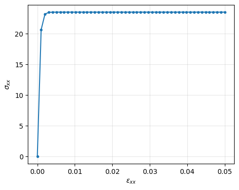
../../../../_images/17e1b2b271d5605b25efb55144057498514cf2a3f8e4258a520d5be2c8e2d25e.png

The initial linear segment is purely elastic. Once the von Mises stress exceeds the yield surface the Perzyna flow rule activates and the stress plateaus at the rate-dependent overstress level — a textbook perfect-viscoplastic response.

Saving the trajectory to disk#

The full result dict can be saved to a single .pt file, keyed by the same strings driver.result() returns in memory:

driver.save_result("result.pt")

loaded = torch.load("result.pt", weights_only=True)
print("entry count:", len(loaded))
print("a few keys :", list(loaded)[:4])

entry count: 295
a few keys : ['input.0.t', 'input.0.E', 'input.1.t', 'input.1.E']

Where to go next#

To prescribe stress instead of strain, swap which variable the prescribed_* block supplies; the rest of the workflow is unchanged.
Give prescribed_time and the prescribed tensors a trailing batch axis and the driver will sweep that axis in parallel — useful for parameter or initial-condition sweeps. See Vectorization for the batching rules.
For gradient-based training through a transient response, see pyzag.